Download

1 / 110
1.1k likes | 1.26k Views
Design and Analysis of Algorithms. Rahul Jain. Grading : 50 marks for final exam 35 marks for midterm exam 10 marks for two quizzes (5 marks each) 5 marks for tutorial participation Tutorials : Start next week. Information available at course home page

E N D
Design and Analysis of Algorithms Rahul Jain
Grading : 50 marks for final exam 35 marks for midterm exam 10 marks for two quizzes (5 marks each) 5 marks for tutorial participation Tutorials : Start next week. Information available at course home page Acknowledgment : We thank Prof. Sanjay Jain for sharing with us his course material. Lecturer : RAHUL JAIN Office : S15-04-01 Email: rahul@comp.nus.edu.sg Phone: 65168826 (off) Tutors : ERICK PURWANTO (erickp@comp.nus.edu.sg) ZHANG JIANGWEI (jiangwei@nus.edu.sg) Prerequisites : (CS2010 or its equivalent) and (CS1231 or MA1100) Book : Title : Algorithms Authors : R. Johnsonbaugh and M. Schaefer Publication : Pearson Prentice Hall, 2004 (International Edition) Other reference books mentioned in the course home page : http://www.comp.nus.edu.sg/~rahul/CS3230.html
Regarding CS3230R According to my information current implementation of the R-modules is as follows: • Discuss with the lecturer that you would like to do the R-module. • The lecturer will decide whether it is appropriate for you after teaching you for a period (around middle of semester or end of semester). • Start work on it after the lecturer has decided (middle of the current semester or at the next semester). The course will be registered only in the following semester.
What we cover in the course Greedy Algorithms • Kruskal’s algorithm for Minimum Spanning Tree • Prim’s algorithm for Minimum Spanning Tree • Dijkstra’s algorithm for finding shortest path between a pair of points in a graph • Huffman codes • The continuous Knapsack problem • Dynamic Programming • Computing Fibonacci numbers • Coin changing • The algorithm of Floyd and Warshall Sorting/Searching/Selection • A lower bound for the sorting problem • Counting sort and Radix sort • Topological sort of graphs Divide and Conquer • A Tiling problem • Strassen’s Matrix Product Algorithm • Finding closest pair of points on the plane
What we cover in the course • P v/s NP • Polynomial time, Non-deterministic algorithms, NP • Reducibility and NP-completeness, NP complete problems • How to deal with NP hard problems • Brute force • Randomness • Approximation • Parameterization • Heuristics Assume familiarity with : • Basic data structures like Stacks, Queues, Linked lists, Arrays, Binary Trees, Binary Heaps, • Basic sorting algorithms like Heap sort • Basic search algorithms like Depth-First search, Breadth-First search • Basic mathematical concepts like Sets, Mathematical Induction, Graphs, Trees, Logarithm
What is an Algorithm ? AbūʿAbdallāhMuḥammadibnMūsāal-Khwārizmī (c. 780 – c. 850) A Persian mathematician, astronomer and geographer. Properties : • Input • Output • Precision • Determinism (exceptions: randomization, quantum etc.) • Finiteness • Correctness • Generality Pseudocode : Has precision, structure, universality. It is unambiguous, clear enough (not too rigorous, will not be concerned with semi-colons, uppercase, lowercase etc.) Analysis : • Correctness • Termination • Time analysis • Space analysis
Pseudocode - Example Algorithm for finding maximum element in an array ----------------------------------------- if (condition) action 1 else action 2 ----------------------------------------- do { action } while (condition) ---------------------------------------- for var = init to limit action ----------------------------------------- for var = init downto limit action -----------------------------------------
Algorithm analysisWorst case, Average case Worst case analysis : t(n) = Maximum units of time taken by the algorithm to terminate for an input of size n. Average case analysis : t(n) = the average units of time taken by the algorithm to terminate for an input of size n. Similar analysis can also be done for space required by the algorithm. The worst case and average case times of the algorithm on an array of size n are each constant * (n-1) since the while loop is always executed (n-1) times, and every other operation takes constant time.
With today’s lecture and the material covered in pre-requisite courses we have covered Chapters 1, 2, 3, 4 from the book.
Divide and Conquer • If the problem is small solve it directly. • If the problem is big, divide it into subproblems. Solve the subproblems, again using divide and conquer. • Combine the solutions of the subproblem to get the solution of the original problem.
Idea of the algorithm • Divide the problem of size n by n into four subproblems each of size n/2 by n/2. • Place one tromino at the centre to create missing cells in each subproblem. • Solve the subproblems using recursion. • 2 by 2 problem is solved directly.
Time Analysis • Chu and Johnsonbaugh (1986) showed that if n ≠ 5, and n2 - 1 is divisible by 3 then the n by n deficient board can be tiled using trominoes. • Some 5 by 5 boards can be tiled and some cannot.
Idea of the algorithm • Divide the array of size n into two arrays of size n/2. • Sort the two subarrays using recursion. • Merge the two sorted parts using subroutine merge.
Mergesort – Time Analysis Stable sort: A sorting algorithm is stable if the relative positions of items with duplicate values are unchanged by the algorithm. Mergesort is stable.
Idea of the algorithm • Divide the problem of multiplying two n by n matrices into the problem of multiplying 7, n/2 by n/2 matrices (you also do constant number of additions of n/2 by n/2 matrices). • Use recursion to solve the subproblems.
Idea of the algorithm • Divide the set of n points on the plane into two halfs (using x-coordinate). • Find the shortest distance between pairs of points in the two halfs using recursion. Let delta be their minimum. • Consider a strip of size 2 times delta in the middle of the two halfs. • Sort the points in this strip using y-coordinate (this can be done only using merge since the subparts are already sorted according to y-coordinate). • Start from bottom and compare each point with the next seven points to identify the closest pair (this works because in each box that we considered there can be at most 8 points).
What we did last time Divide and conquer: • Tiling problem • Mergesort • Strassen’s matrix product • Finding closest pair of points on a plane
Idea of the algorithm • Assume that the elements of the array arrive one by one. • Keep inserting them at the right place in the current subarray which is already sorted. • Nice property: It is an online algorithm.
Quicksort The algorithm ‘partition’ inserts val at the index h such that values less than val are on the left of index h and values at least val are on the right of h. Quicksort Algorithm
Randomized Quicksort Randomized Quicksort
Idea for partition algorithm • Let the current stage of array be like : F SSSSLLLL C RRRRR • F is first element, S < F, L ≥ F, C is the current element, R is rest of the elements. • If current element C ≥ F, then don’t do anything, just let next element on right to be C. • If C < F, then swap C with first L, and let next element on right to be C. • At the end swap F with the last S element.
Idea of the algorithms • Take an element of the array (of value val) and place it at the right index h. Elements to the left of h are less than val and to the right are greater than or equal to val (partition algorithm). • Recursively sort a[i] … a[h-1] and a[h+1] … a[j] • In normal quicksort, the element is taken to be the first element of the array. • In randomized quicksort, the element is randomly chosen among all elements. Quicksort is quite good in practice that is why ‘quicksort’. No extra array is needed. Quicksort is not stable.
A lower bound for comparison based algorithms The worst case time of a comparison based sorting algorithm is Ω(n log n). Proof done in class. Idea: Any comparison based algorithm will have a decision tree, with n! leaves (for n bit inputs). Height of this tree is Ω(n log n). A decision tree for the comparison based algorithm is a binary tree with the nodes representing comparisons (a < b?), the left subtree represents the continuation of the algorithm on the result of comparison being yes and the right subtree represents the continuation of the algorithm on the result of comparison being no.
Counting Sort • Not a comparison based algorithm, uses some information about the inputs i.e. the elements are numbers from 0 to m. • Running time is linear, lower bound of Ω(n log n) does not apply.
Time analysis • Since each loop runs in time θ(m) or θ(n), the running time is θ(m + n). Idea of algorithm • First make sure that c[k] = number of occurrences of value k in input array a. • Then make sure that c[k] = number of occurrences of value less than or equal to k in input array a. • Produce sorted array b using c. • Copy b back to a. Counting sort is stable (done in tutorial).
Radix Sort Idea of algorithm: Starting from the least significant digit, sort using counting-sort. Correctness of the algorithm shown in class. Running time is done in tutorial. Radix sort was originally used to sort punch cards.
(Random) Selection Finding median is a special case of this.
Idea of algorithm • Using random-partition, get location p (note that everything to the left of p will be smaller than the value at p and everything to the right will be at least the value at p.) • If k = p then stop. • If k < p, act recursively on the left of p. • Else act recursively on the right of p. Running Time : The expected running time is θ(n). Proof done in class. Idea similar to the analysis of random-partition. When element is selected randomly, p is near middle (in expectation). • The worst case time of random-select isθ(n2) (done in tutorial). • Any deterministic algorithm solving selection must take time at least n. • Deterministic algorithm due to Blum, Floyd, Pratt, Rivest and Tarjan (1973) runs in time θ(n).
What we did last time • Selection sort • Quicksort • Lower bound for comparison based algorithms • Couting sort, Radix sort (not comparison based) • Random Selection
Greedy Algorithms Greed is Good !
Coin Changing • The algorithm is not optimal for denominations {1,6,10}.
Optimality for {1,5,10} The algorithm is optimal for denominations {1,5,10} for every input amount A. Idea: use mathematical induction. • Let greedy(A) represent the number of coins used by the greedy algorithm for input amount A. • Let optimal(A) represent the optimal number of coins for amount A. • Can verify by direct calculation for A = 1, 2, … , 9, that greedy(A) = optimal(A). • Let A ≥ 10. Then by induction hypothesis: greedy(A-10) = optimal(A-10). • Note that greedy(A) = 1+ greedy(A-10). • Also note that optimal(A) = 1 + optimal(A-10) (since optimal solution must use at least one 10 dollar coin for A ≥ 10). • Hence greedy(A) = optimal(A). What goes wrong with {1,6,10} in this argument ?
Kruskal’s Algorithm Kruskal’s algorithm finds a minimal spanning tree in a connected, weighted graph G with vertex set {1, …, n}. A spanning tree is a tree T such that every pair of vertices are connected via edges in T. A minimal spanning tree is a spanning tree such that the sum of the weights of all its edges is the least among all spanning trees. Note: A forest with (n-1) edges is a spanning tree. Idea (Greedy approach): • Start with S having no edges. • Add an edge of minimum weight not contained in S, to S, such that S does not contain a cycle. • Keep doing this till S contains n-1 edges. • At the end since S is a forest with n-1 edges, it must be a spanning tree.