Download
1 / 54
690 likes | 1.21k Views
THE UNIVERSITY OF BIRMINGHAM. CHM2S1-A Intermolecular Forces Dr R. L. Johnston. Handout 1: Introduction to Intermolecular Forces I: Introduction Evidence for Intermolecular Forces The nature of Intermolecular Forces Electric Multipoles II: Intermolecular Interactions

E N D
THE UNIVERSITY OF BIRMINGHAM CHM2S1-A Intermolecular ForcesDr R. L. Johnston Handout 1: Introduction to Intermolecular Forces I: Introduction • Evidence for Intermolecular Forces • The nature of Intermolecular Forces • Electric Multipoles II: Intermolecular Interactions • Types of Intermolecular Interactions • Many-Body Energies • Total Energy • Comparison of Intermolecular Forces
Overview • Intermolecular forces are critically important in determining the properties of matter. • We will discuss the forces that exist between atoms and molecules. • Evidence (taken from thermodynamic, structural and other experimental studies) will be provided for the existence of intermolecular forces. • The various types of intermolecular forces will be described: including the origin of the forces and their distance-dependence. • A more detailed discussion of the consequences and implications of intermolecular forces will follow. • Finally, the “anomalous” properties of water and the importance of hydrogen bonding and the “hydrophobic effect” in biological systems will be analysed.
Learning Objectives • To recognise the importance of intermolecular forces in determining the physical properties of matter; • To know the experimental evidence for the existence of intermolecular forces; • To understand the origins of the various types of intermolecular forces; • To know the distance-dependence of intermolecular forces of various types; • To understand the origins of the so-called “anomalous” properties of water. • To recognise the importance of hydrogen bonding and the hydrophobic effect in biological systems.
References Fundamentals • P. W. Atkins, The Elements of Physical Chemistry (3rd edition), OUP, Oxford, 2000. • P. W. Atkins, J. de Paula, Atkins' Physical Chemistry (7th edition), OUP, Oxford, 2001. • K. A. Dill, S. Bromberg, Molecular Driving Forces, Garland Science, New York, 2003. More Advanced • M. Rigby, E. B. Smith, W. A. Wakeham, G. C. Maitland, The Forces Between Molecules, OUP, Oxford, 1986. • A. J. Stone, The Theory of Intermolecular Forces, OUP, Oxford, 1997.
1. Evidence for Intermolecular Forces • Solid and Liquid States of Matter – In the absence of interatomic or intermolecular forces, all matter would exist in the gas form, even at 0K! • Gas Imperfection – The failure of real gases to obey the perfect/ideal gas equation of state (PV = nRT). • Non-Ideal Mixtures / Solutions – e.g. Deviations from Raoult’s Law for an A-B mixture are due to different strengths of the A–A, B–B and A–B intermolecular forces. • Transport Properties of Dilute Gases – The transport of momentum, energy or mass through a dilute gas, under the influence of a gradient of velocity, temperature or concentration, is affected by molecule-molecule collisions. The corresponding transport coefficients (shear viscosity, thermal conductivity, diffusion) are directly related to the intermolecular forces between the gas molecules.
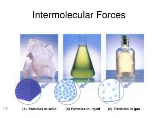
States of Matter • Solids: Kinetic Energy (KE) of atoms/molecules small compared to strength of intermolecular interaction energies (KE Uinter). small amount of movement around equilibrium positions regular crystalline structures usually adopted (long range order) doesn’t take shape of or fill a container very low compressibility • Liquids:KE Uinter atoms/molecules can move around (diffusion) on average, some local order exists takes shape of (but doesn’t fill) a container low compressibility • Gases:KE Uinter atoms/molecules move quite freely less frequent collisions than in liquids takes shape of and fills a container high compressibility
2. The Nature of Intermolecular Forces 2.1 Intermolecular Interactions • The interaction energy (Uinter) between two particles (atoms or molecules) is defined as the pair potential (energy), U(r), which depends on the intermolecular separation, r. • The force, F(r), between the two particles is obtained as the negative of the gradient of the pair potential: • At very large separations (as r), the interparticle interaction is negligible (U0, F0). • At shorter separations, the particles attract (F < 0, particles pulled together). The dimer is more stable than the two isolated particles, hence U(r) < 0. • At very short separations (r0), the particles repel each other (F > 0, particles pushed apart). • At r = re, U(r) is at its minimum (Umin) and the interparticle force, F = 0.
0 Umin
2.2 Note on Terms Adopted • Instead of talking about particles and interparticle forces etc., in this course we will refer to molecules and Intermolecular Forces (IMFs), though some of these interactions can also apply to atoms. • Although we refer to Intermolecular Forces, in the following discussion of types of IMFs, their origin and their range (distance-dependence), we will actually refer to the intermolecular potential energy function, U(r), rather than the force F(r). • Note: the previous diagram showed the total potential energy between 2 molecules. We are now going to discuss the various contributions to this total energy.
2.3 Long- and Short-Ranged Interactions • IMFs can be divided into two classes: long-ranged and short -ranged, according to the dependence of the potential energy U on the separation r. • For a particular type of IMF, the intermolecular potential energy function is generally modelled by a power law in r : (where C is a constant). • Long-ranged interactions: 6 e.g. Coulombic U(r) 1/r dispersion U(r) 1/r6 • Short-ranged interactions: 6 or ere.g. exchange repulsion • Attractive interactions:U(r) < 0 • Repulsive interactions:U(r) > 0
+ q +q 3. Electric Multipoles 3.1 Definitions • Monopole: a point charge (e.g. Na+, Cl). • Dipole:an asymmetric charge distribution in a molecule, where there is no net charge but one end of the molecule is negative (partial charge = q) relative to the other (partial charge = +q). • Molecules may possess higher order electric multipoles, arising from their non-spherical charge distributions. • Each type of multipole has an associated multipole moment: the monopole moment is the charge of the atom/molecule; the dipole moment is a vector whose magnitude is the product of the charge and distance between the charge centres. Higher order multipole moments have tensor properties.
q +q 3.2 Molecular Dipoles • A polar molecule is one which possesses a permanent dipole moment:there is an asymmetric charge distribution, with one end of the molecule relatively negative (q) with respect to the other (+q). NB:q is a multiple of e(q = ae) but a doesn’t have to be an integer and may be less than 1). • Examples: FCl (where the F atom is negative with respect to the Cl atom) and the polyatomic molecule HCCl3 (where the H end of the molecule is positive with respect to the three Cl atoms). • The magnitude of the dipole moment (which by definition points from the negative toward the positive end) is given by = q, where is the distance between the centres of the two opposite charges.
H b1 O Cl b2 H Cl b b Cl Cl O C O • The dipole is a vector quantity: the total molecular dipole () for a polyatomic molecule can be obtained by summing the vectors corresponding to bond dipoles (b) pointing along each bond: • For 2 equal bond dipoles (b) at an angle to each other, the resultant total molecular dipole () is given approximately by: • Sometimes bond dipoles cancel out, so that the molecule as a whole has no dipole moment:
3.3 Higher Multipoles • Although the linear molecules CO2 (O=C=O) and acetylene (HCCH) and the planar molecule benzene (C6H6) do not have dipole moments, they have non-zero quadrupole moments. • For more symmetrical molecules, the first non-zero multipole moments have higher order: thus, the methane molecule (CH4) has no dipole or quadrupole moment, but it has a non-zero octopole moment.
Dipole moments () and polarizability volumes ( = /40) for some atoms and molecules (1D (1 Debye) = 3.3361030 C m).
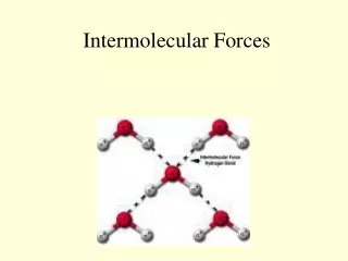
4. Types of Intermolecular Interactions 4.1 Overview Electrostatic: interactions between charged atomic or molecular species (ions = monopoles) or between asymmetric charge distributions (dipoles, quadrupoles etc.) in neutral molecules. Induction: an electric charge (monopole) or higher multipole causes polarization of neighbouring atoms/molecules and induced multipoles. The attractive interaction between the original multipole and the induced multipole gives rise to the induction energy. Dispersion: attractive interactions between instantaneous dipoles (and higher multipoles) arising due to fluctuating charge distributions in atoms and molecules. Hydrogen Bonding: attractive interactions of the form XHY – a hydrogen atom is covalently bound to one electronegative atom (X = N, O, F etc.) and interacts with a second electronegative atom (Y).
Electrostatic interactions can be attractive or repulsive, depending on ionic charges and the orientation of the molecular multipoles. • The range of the interaction energies depends on the type of interaction. • van der Waals forces: a term used to cover electrostatic, induction and dispersion interactions between discrete neutral molecules or atoms. The most important contributions have 1/r 3 or 1/r 6 distance dependence. • These IMFs should be contrasted with covalent bonds, where molecules are bound by the sharing of electrons. Covalent bonds are typically much stronger than IMFs.
4.2 Short-Ranged Repulsions • There is a limit to the compressibility of matter, due to repulsive interactions (due to overlap of electron densities) which dominate at short range. • At short internuclear separations there are electrostatic repulsions between the atomic nuclei, as well as between the electrons (both valence and core) on neighbouring atoms. • There is also a short range Pauli or Exchange Repulsion between the electrons on neighbouring atoms, which is quantum mechanical in origin and derives from the Pauli exclusion principle. • The total short range repulsive interaction is generally modelled by a steep 1/r n (where n is usually 12) dependence on interatomic distance, though an exponential (er) dependence is more accurate.
Q1 Q2 r 4.3 Electrostatic Energy Ion-Ion (Coulomb) Energy • The interaction of two stationary point charges (Q1 and Q2), separated by a distance ris given by the Coulomb potential energy: where Q = ne (n is an integer and e is the magnitude of the charge on an electron = 1.602 1019 C), r is in metres and 0 ( = 8.8541012 J1 C2 m1) is the vacuum permittivity. • Note: like charges (+ + or ) repelUC(r) > 0 opposite charges (+ ) attractUC(r) < 0 • The Coulomb interaction ( r1) is very long-ranged – it falls off very slowly with distance.
dielectric vacuum 0 r r Dielectric Constant • In a dielectric medium, the vacuum permittivity (0) is replaced by the permittivity of the medium (), where: =0.r • r is the relative permittivity (since r = /0) – also known as the dielectric constant. • Highly polar solvents have high dielectric constants r • e.g. r (H2O) = 78 • This leads to a large reduction in the Coulombic potential between ions in polar solvents.
+Q1 q +q 2 r Q1 q +q 2 Ion-Dipole Energy • The interaction energy between a stationary point charge Q1and a permanent dipole 2, separated by a distance r(for the most stable arrangements shown below)is given by: where Q1 (= ne) has units of C and 2(= q)has units of C m. • Note: the interaction energy now depends upon the orientation of the dipole relative to the point charge (and the sign of the charge).
1 r 2 3 Dipole-Dipole Energy • When two polar molecules are close to each other there is a tendency for their dipoles to align, with the attractive head-to-tail arrangement (1) being lower in energy than the repulsive head-to-head or tail-to-tail arrangements (2 and 3). • The energy of interaction of two co-linear dipoles (1 and 2), arranged in a head-to-tail fashion, is given by: where r is the distance between the centres of mass of the two molecules.
2 1 • The potential energy of interaction between two parallel dipoles which are not co-linear (i.e. where the inter-molecular vector makes an angle to the intra-molecular bonds) is given by: • For general intermolecular geometries, a function of the three angles that define the relative orientations of the two dipoles, must be included. [See workshop question.] • In the side-on arrangement, antiparallel dipoles (1) are favoured energetically over parallel dipoles (2).
The alignment of molecular dipoles is opposed by the effect of thermal energy, which leads to rotation of the dipoles. • At temperatures where the thermal energy (kT) is greater than the electrostatic dipole–dipole interaction energy (UDD), the rotationally averaged energy of interaction between two dipoles 1 and 2, separated by a distance r, can be obtained from a Boltzmann-weighted average: • Note: the rotationally averaged dipole-dipole interaction is shorter-ranged than when the dipoles are static!
At room temperature (T = 300 K), this gives: where the dipole moments are in Debye (1 D = 3.3361030 C m). • Example: at room temperature, two molecules with dipole moments of 1 D (e.g. HCl), at a separation of r = 0.3 nm, have an average dipole–dipole interaction energy of approximately 1.4 kJ mol1. • Due to the r6 distance dependence, doubling the distance reduces the interaction energy by a factor of 26 (64).
Multipole-Multipole Interactions • The electrostatic interaction between higher order multipoles can be treated in an analogous fashion to that described above for dipole–dipole interactions. • The distance-dependence of the interaction energy between an n-pole and an m-pole (assuming no molecular rotation) is given by: where n and m are the orders of the multipoles: n,m = 1 (monopole), 2 (dipole), 3 (quadrupole), 4 (octopole) … • Examples: • monopole-monopole (coulomb) U(r) r 1 • monopole-dipole U(r) r 2 • dipole-dipole U(r) r 3 • dipole-quadrupole U(r) r 4 • quadrupole-quadrupole U(r) r 5 • Note: The higher the order of the multipole, the shorter-ranged the interaction (the more rapidly it falls off with distance).
Quadrupole-Quadrupole Interactions • In cases where quadrupolar interactions dominate, T-shaped intermolecular geometries are generally adopted, with the positive regions of one quadrupole being attracted to the negative regions of another. • Example: the benzene dimer (C6H6)2, which has a T-shaped geometry (a) where one CH bond of one molecule is oriented towards the -electron cloud of the other. (In the benzene molecule, the ring C atoms are relatively negative with respect to the H atoms.) • However, the quadrupole in perfluorobenzene (C6F6) is the opposite way round to that of benzene (i.e. the peripheral F atoms carry more electron density than the C atoms of the ring). Therefore, the mixed dimer (C6H6)(C6F6) has a . -stacked geometry (b), with parallel rings.
r q +q Q1 + + + + ind 2 4.4 Induction Energy • A charge (i.e. an ion = electric monopole), or asymmetric charge distribution (dipole, quadrupole etc.) gives rise to an electric field (E) which causes the polarization of neighbouring atoms or molecules and the creation of an induced dipole, ind = (where is the polarizability of the atom or molecule). Ion-Induced Dipole Energy
r q2 q1 +q2 +q1 1 ind Dipole-Induced Dipole Energy • The induced dipole (ind) interacts in an attractive fashion with the original (permanent) dipole (1). • The (induction) interaction energy between a permanent dipole (1) on molecule 1 and an induced dipole on molecule 2 (which has no dipole but has polarizability 2), at a distance r, is given by: where 2 is the polarizability volume of molecule 2 (2 = 2/(40)).
As the direction of the induced dipole follows that of the permanent dipole, the effect survives even if the permanent dipole is subject to thermal reorientations. • The above equation can be rewritten as: • Example: For a polar molecule with 1 D (e.g. HCl), at a distance r = 0.3 nm from a non-polar molecule with polarizability volume 101030 m3 (e.g. benzene), the dipole–induced–dipole interaction energy is approximately 0.8 kJ mol1.
Note: if both molecules are polar, then they will induce dipoles in each other. • Note: this induction energy is in addition to the electrostatic interaction energy, UDD(r), between the two permanent dipoles. • Dipoles (and higher multipoles) can also be induced by neighbouring molecules with permanent charges (monopoles) or high-order multipoles, and similar expressions can be derived for the interactions between these permanent and induced multipoles.
r 4.5 Dispersion Energy • The intermolecular forces between nonpolar molecules and closed shell atoms (e.g. rare gas atoms He, Ne, Ar …) is dominated by “London” or dispersion forces. • The dispersion energy contributes to the intermolecular interactions between all pairs of atoms or molecules. It is also generally the dominant contribution, even for polar molecules. • Long range attractive dispersion forces arise from dynamic electron correlation: fluctuations in electron density give rise to instantaneous electronic dipoles (and higher multipoles), which in turn induce dipoles in neighbouring atoms or molecules. • The instantaneous dipoles are correlated so they do not average to zero.
A general expansion for the attractive energy (Udisp(r)) due to these dispersion forces can be written: where the terms Cn are constants and r is the interatomic distance. • The first term represents the instantaneous dipole–dipole interaction and is dominant, so the higher terms (which contribute less than 10% of the total dispersion energy) are often omitted when calculating dispersion energies. • A reasonable approximation to the dispersion energy is given by the London formula (derived by London, based on a model by Drude), in which the dispersion energy between two identical atoms/molecules is given by: where , and I are the polarizability, polarizability volume and ionization energy of the atom/molecule.
The 2 term arises because the magnitude of the instantaneous dipole depends on the polarizability of the first atom/molecule and the strength of the induced dipole (in the second atom/molecule) also depends on . • Example: the (rotationally averaged) dispersion energy of interaction between two CH4 molecules ( = 2.61030 m3, I = 700 kJ mol1), at a separation of r = 0.3 nm, is approximately 5 kJ mol1. • The dispersion energy between two unlike molecules (with polarizability volumes 1 and 2 and ionization energies I1 and I2) is given by:
The Lennard-Jones Potential • Taking into account both repulsive and attractive (dispersion) interactions, a good approximation to the total potential energy of interaction between two neutral atoms or non-polar molecules is given by the Lennard-Jones (LJ) potential: where is the depth of the energy well and is the separation at which ULJ(r) = 0. • The equilibrium separation (the position of the minimum in ULJ(r)) occurs at re = 21/6. [ULJ(re) = .] • Note: due to the r6 dependence of the attractive term, the LJ potential has also been used to approximate the interaction energy between rotating dipoles.
The Lennard-Jones Potential ULJ +r 12 ULJ r 6
Table of LJ well depths () for rare gas dimers and boiling temperatures (Tb) and melting temperatures (Tm) of the rare gas elements.
The increase in on going to heavier rare gases reflects the increase in the attractive dispersion forces because of the higher polarizability due to the lower effective nuclear charge experienced by the outer electrons in the heavier rare gas atoms. • The boiling temperatures (Tb) of the rare gas elements follows the same trend as that observed for the values of the dimers (i.e. increasing with increasing atomic number) because of the increasing dispersion forces. • The same trend is observed for the melting temperatures (Tm) of the rare gas elements. • Note: helium cannot be solidified at pressures lower than 25 atmospheres.
n-pentane Tb = 309.4 K neo-pentane Tb = 282.7 K • As molecules are larger and (usually) more polarizable than rare gas atoms, typical binding energies due to dispersion forces are of the order 10 kJ mol1 per intermolecular interaction—i.e. (Mol2) 10(Rg2). • Example: the magnitude of the dispersion energy for two methane molecules separated by 0.3 nm is approximately 4.7 kJ mol1 (i.e. 4.7 kJ mol1). • Comparing isomers of alkane molecules, straight chain isomers generally have higher boiling/melting points, due to increased dispersion forces (larger instantaneous dipoles and shorter intermolecular distances)
4.6 Hydrogen Bonding Definition • A hydrogen bond is an intermolecular linkage of the form XHY, where a hydrogen atom is covalently bound to one electronegative atom (X = N, O, F etc.) and interacts with a second electronegative atom (Y), which has an accessible lone-pair of electrons. XHhydrogen bond donor. Yhydrogen bond acceptor. Characteristic properties of hydrogen bonds: • hydrogen-bonding is directional (depends on bond orientations) and short-ranged. • the XHY angle is normally close to 180; the HY distance is significantly longer than a HY covalent bond; • lengthening of the XH bond; • large red-shift of the XH stretching vibration; • broadening and gain of intensity of the XH stretch; • deshielding of the hydrogen-bonded proton (observed as a shift in its NMR signal). • typical hydrogen bond strengths lie in the range 10–25 kJ mol1.
Contributions to Hydrogen Bonding • The major component (probably around 80%) is electrostatic, as a H atom bonded to an electronegative atom (X), will carry a significant fractional positive charge (+q) which will undergo an attractive interaction with the fractional negative charge (q) on the neighbouring electronegative atom (Y). • Other important contributions come from induction and dispersion forces, as well as from charge transfer—which can be regarded as incipient covalent bond formation—from atom Y to the hydrogen atom. • Example: contributions to the interaction energy between two water molecules, at the equilibrium geometry (in kJ mol1):
Consequences of Hydrogen Bonding • The anomalously high boiling points of ammonia, water and hydrogen fluoride can be attributed to the occurrence of hydrogen bonding, which is significantly stronger for these elements than for their heavier congeners. • The tetrahedral three-dimensional structure of ice and the local structure of liquid water is a consequence of hydrogen bonding, as is the fact that ice is less dense than water! • The existence of life on Earth is a direct consequence of the hydrogen bonding present in water and the high range (100C) over which water remains liquid. • Hydrogen bonding plays a very important role in biology, being responsible for the structural organization of proteins and other bio-molecules and governing crucial in vivo proton-transfer reactions.
5. Many-Body Energies • On moving from dimers to larger aggregations of atoms (clusters), or to the bulk liquid or solid phase, accurate modelling of the interatomic forces between the rare gases requires the addition of non-pairwise additive many-body energies. • Even for a rare gas trimer (Rg3), the total potential energy is not just the sum of the three pair interactions: UabcUab + Ubc + Uca. • This non-pair-additivity reflects the fact that the dispersion attraction between two atoms is modified by the presence of other neighbouring atoms. • [Note: induction energies are also non-pair-additive because the polarization of an atom/molecule by an ion/dipole etc. will be affected by the presence of any other ions or dipoles nearby.]
c rbc c rca b a a b rab a b c c a b • The major correction to the dispersion energy due to many-body interactions is the Axilrod-Teller (3-body) potential: UAT < 0 Linear arrangement: introduction of cincreases attraction between a and b. UAT > 0 Triangular arrangement: introduction of cdecreases attraction between a and b.
In condensed phases (liquids and solids), maximisation of the pair-wise additive van der Waals energies usually leads to close-packed-type structures with a large number of triangles. Therefore, the many-body energy (UAT) is usually positive (leading to a decrease in the total interaction energy). • For the rare gases, the many-body energy is generally small, accounting for only 10% of the total interaction energy in liquid or solid argon, for example. In the gas phases the effect is even smaller. • For non-spherical molecules, UAT will depend on the relative orientations of the molecules, as well as their positions. • Many-body forces are large for metals and semiconductors, both in the liquid and the solid phases.
6. Total Energy • In many cases, more than one types of intermolecular force may be in operation, depending upon whether the molecules carry a net charge or possess permanent multipole moments. • The total potential energy is given by the sum of the short-range repulsive energy and the longer-ranged attractive energy. For neutral molecules, these attractive components correspond to van der Waals and (where appropriate) hydrogen-bonding energies: Utot = Urep + UvdW + UHB • (Ignoring any small many-body effects) this yields the familiar pair potential curve for Utot(r).
7. Comparison of Intermolecular Forces • With the exception of small, highly polar molecules (such as H2O), the dispersion energy is the largest contribution to intermolecular bonding between uncharged molecules. • Induction energies are small unless one of the molecules is charged. • Note: intermolecular forces (vdW energies typically < 30 kJ mol1) are much weaker than the covalent bonds (typically hundreds of kJ mol1) within molecules:
Distance-dependence and typical magnitudes of different types of IMF