Download
1 / 38
450 likes | 1.63k Views
Grain Boundaries. In the last four lectures, we dealt with point defects (e.g. vacancy, interstitials, etc.) and line defects (dislocations). There is another class of defects called interfacial or planar defects : They occupy an area or surface and are therefore bidimensional.

E N D
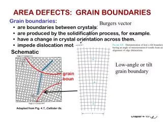
In the last four lectures, we dealt with point defects (e.g. vacancy, interstitials, etc.) and line defects (dislocations). • There is another class of defects called interfacial or planar defects: • They occupy an area or surface and are therefore bidimensional. • They are of great importance in mechanical metallurgy. • Examples of these form of defects include: • grain boundaries • twin boundaries • anti-phase boundaries • free surface of materials • Of all these, the grain boundaries are the most important from the mechanical properties point of view.
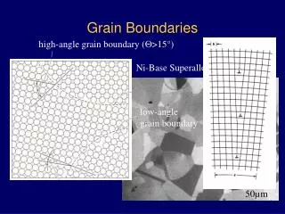
Crystalline solids (most materials) generally consist of millions of individual grains separated by boundaries. • Each grain (or subgrain) is a single crystal. • Within each individual grain there is a systematic packing of atoms. Therefore each grain has different orientation (see Figure 16-1) and is separated from the neighboring grain by grain boundary. • When the misorientation between two grains is small, the grain boundary can be described by a relatively simple configuration of dislocations (e.g., an edge dislocation wall) and is, fittingly, called a low-angle boundary.
Figure 16.1. Grains in a metal or ceramic; the cube depicted in each grain indicates the crystallographic orientation of the grain in schematic fashion
When the misorientation is large (high-angle grain boundary), more complicated structures are involved (as in a configuration of soap bubbles simulating the atomic planes in crystal lattices). • The grain boundaries are therefore: • where grains meet in a solid. • transition regions between the neighboring crystals. • Where there is a disturbance in the atomic packing, as shown in Figure 16-2. • These transition regions (grain boundaries)may consist of various kinds of dislocation arrangements.
Figure 16.2. At the grain boundary, there is a disturbance in the atomic packing.
In general, a grain boundary has five degrees of freedom. • We need three degrees to specify the orientation of one grain with respect to the other, and • We need the other two degrees to specify the orientation of the boundary with respect to one of the grains. • Grain structure is usually specified by giving the average diameter or using a procedure due to ASTM according to which grains size is specified by a number n in the expression N = 2n-1, where N is the number of grains per square inch when the sample is examined at 100x.
Tilt and Twist Boundaries • The simplest grain boundary consists of a configuration of edge dislocations between two grains. • The misfit in the orientation of the two grains (one on each side of the boundary) is accommodated by a perturbation of the regular arrangement of crystals in the boundary region. • Figure 16.3 shows some vertical atomic planes termination in the boundary and each termination is represented by an edge dislocation.
Figure 16-3(b). Diagram of low-angle grain boundary. (a) Two grains having a common [001] axis and angular difference in orientation of (b) two grains joined together to form a low-angle grain boundary made up of an array of edge dislocations.
The misorientation at the boundary is related to spacing between dislocations, D, by the following relation: where b is the Burgers vector. • As the misorientation q increases, the spacing between dislocations is reduced, until, at large angles, the description of the boundary in terms of simple dislocation arrangements does not make sense. (for q very small) (16-1)
For such a case, becomes so large that the dislocations are separated by one or two atomic spacing; • the dislocation core energy becomes important and the linear elasticity does not hold. • Therefore, the grain boundary becomes a region of severe localized disorder. • Boundaries consisting entirely of edge dislocations are called tilt boundaries, because the misorientation, as can be seen in Figure 16.3, can be described in terms of a rotation about an axis normal to the plane of the paper and contained in the plane of dislocations.
The example shown in figure 16.3 is called the symmetrical tilt wall as the two grains are symmetrically located with respect to the boundary.
A boundary consisting entirely of screw dislocations is called twist boundary, because the misorientation can be described by a relative rotation of two grains about an axis. • Figure 16.4 shows a twist boundary consisting of two groups of screw dislocations. • It is possible to produce misorientations between grains by combined tilt and twist boundaries. In such a case, the grain boundary structure will consist of a network of edge and screw dislocations.
Calculation of the Energy of a Grain Boundary • The dislocation model of grain boundary can be used to compute the energy of low-angle boundaries (q< 10o). • For such boundaries the distance between dislocations in the boundary is more than a few interatomic spaces, as: (16-2)
Consider a tilt boundary consisting of edge dislocations with spacing D. Let us isolate a small portion of dimension D, as in Figure 16.5, with a dislocation at its center. • The energy associated with such a portion, E, includes contributions from the regions marked I, II, and III in figure 16.5.
Figure 16.5. Model for the computation of grain boundary energy.
EIis the energy due to the material inside the dislocation core of radius rI. • EII is the energy contribution of the region outside the radius and inside the radius R = KD > b, where K is constant less than unity. • In this region II, the elastic strain energy contributed by other dislocations in the boundary is very small. • EII is mainly due to the plastic strain energy strain energy associated with the dislocation in the center of this portion.
EIII, the rest of the energy in this portion, depends on the combined effects of all dislocations. • The total strain energy per dislocation in the boundary is, then, • Consider now a small decrease, , in the boundary misorientation. The corresponding variation in the strain energy is (16-3) (16-4)
(16-5) and • The new dimensions of this crystal portion are shown in Fig. 16-6. • The region immediately around the dislocation, contributing an energy EI , does not change. • This region does not change because EI , the localized energy of atomic misfit in the dislocation core, is independent of the disposition of other dislocations.
Figure 16-6. New dimensions of a portion of crystal after a decrease in the boundary misorientation.
Thus, dEI =0. EII increases by a quantity dEII, corresponding to an increase in R by dR. • EIII, however, does not change with an increase in D, because although the volume of region III increases, the number of dislocations contributing to the strain energy of this region decreases.
Role of Grain Boundaries • Grain boundaries have very important role in plastic deformation of polycrystalline materials. • We outline below the important aspects of the role of grain boundaries. 1. At low temperature (T<0.5Tm, where Tm is the melting point in K), the grain boundaries act as strong obstacles to dislocation motion. Mobile dislocations can pile up against the grain boundaries and thus give rise to stress concentrations that can be relaxed by initiating locally multiple slip.
2. There exists a condition of compatibility among the neighboring grains during the deformation of polycrystals; that is, if the development of voids or cracks is not permitted, the deformation in each grain must be accommodated by its neighbors. • This accommodation is realized by multiple slip in the vicinity of the boundaries which leads to a high strain hardening rate. • It can be shown, following von Mises, that for each grain to stay in contiguity with others during deformation, there must be operating at least five independent slip systems - Taylors Theorem.
This condition of strain compatibility leads a polycrystalline sample to have multiple slip in the vicinity of grain boundaries. • The smaller the grain size, the larger will be the total boundary surface area per unit volume. • In other words, for a given deformation in the beginning of the stress-strain curve, the total volume occupied by the work-hardened material increases with the decreasing grain size. • This implies a greater hardening due to dislocation interactions induced by multiple slip.
3. At high temperatures the grain boundaries function as sites of weakness. • Grain boundary sliding may occur, leading to plastic flow and/or opening up of voids along the boundaries. 4. Grain boundaries can act as sources and sinks for vacancies at high temperatures, leading to diffusion currents as, for example, in the Nabarro Herring creep mechanism. 5. In polycrystalline materials, the individual grains usually have a random orientation with respect to one another.
The term polycrystalline refers to any material which is composed of many individual grains. • However, some materials are actually used in their single crystal state: silicon for integrated circuits and nickel alloys for aircraft engine turbine blades are two examples. • The sizes of individual grains vary from submicrometer (for nanocrystalline structures) to millimeters and even centimeters (for materials especially processed for high-temperature creep resistance). • Figure 16.7 shows typical equiaxed grain configurations for polycrystalline tantalum and titanium carbide.
One example of a material property that is dependent on grain size is the strength of a material; as grain size is increased the material becomes weaker (see Fig.16.8). Note that • strength is expressed in units of stress (MN/m2) • grain size of a material can be altered (increased) by annealing • Hardness measurement (e.g., by vickers indenter) can provide a measure of the strength of the material.
Figure 16.8 The dependence of strength on grain size for a number of metals and alloys.
Grain Size Measurements Grain structure is usually specified by giving the average diameter. Grain size can be measured by two methods. (a) Lineal Intercept Technique: This is very easy and may be the preferred method for measuring grain size. (b) ASTM Procedure: This method of measuring grain size is common in engineering applications.
Lineal Intercept Technique In this technique, lines are drawn in the photomicrograph, and the number of grain-boundary intercepts, Nl, along a line is counted. • The mean lineal intercept is then given as: where L is the length of the line and M is the magnification in the photomicrograph of the material. 10-1
In Figure 16.9 a line is drawn for purposes of illustration. • The length of the line is 6.5 cm. The number of intersections, Nl, is equal to 7, and the magnification M = 1,300. Thus, • Several lines should be drawn to obtain a statistically significant result.
The mean lineal intercept l does not really provide the grain size, but is related to a fundamental size parameter, the grain-boundary area per unit volume, Sv, by the equation • The most correct way to express the grain size (D) from lineal intercept measurements is: • Therefore, the grain size (D) of the material of Figure 10.4 is: 10-2 10-3
ASTM Procedure • With the ASTM method, the grain size is specified by the number n in the expression N = 2 n-1, where N is the number of grains per square inch (in an area of 1 in2), when the sample is examined at 100 power micrograph. Example In a grain size measurement of an aluminum sample, it was found that there were 56 full grains in the area, and 48 grains were cut by the circumference of the circle of area 1 in2. Calculate ASTM grain size number n for this sample.
Solution The grains cut by the circumference of the circle are taken as one-half the number. Therefore,