Download
1 / 29
330 likes | 562 Views
Polynomial functions. Chapter 5. 5.1 – exploring the graphs of polynomial functions. Chapter 5. Polynomial functions. What’s a polynomial?.

E N D
Polynomial functions Chapter 5
5.1 – exploring the graphs of polynomial functions Chapter 5
Polynomial functions What’s a polynomial? A polynomial is any algebraic expression that has several terms, and features addition, subtraction, multiplication and division (but not division by a variable). Examples: We are going to be looking at the graphs of different types of polynomial functions. x + 1 x4 + 5x2 – 4x + 2 Which types have you seen already? linear quadratic x2 – 4x + 6 x3 – 2
Polynomial functions Pull out a graphing calculator.
How graphs work End behaviour: The description of the shape of the graph, from left to right, on the coordinate plane. A Cartesian grid (the x/y-axis) has four quadrants. Example: the graph of f(x) = x + 1 begins in quadrant III and extends to quadrant I.
Domain and range Domain is how much of the x-axis is spanned by the graph. Range is how muhc of the y-axis is spanned by the graph.
Turning points A turning point is any point where the graph changes from increasing to decreasing, or from decreasing to increasing.
Pg. 277, #1-4 Independent practice
5.2 – characteristics of the equations of polynomial functions Chapter 5
example • Determine the following characteristics of each function using its equation. • Number of possible x-intercepts Domain • y-intercept Range • End behaviour Number of possible turning points a) f(x) = 3x – 5 Linear equations (of degree 1) always have only one x-intercept. What’s the degree? The last number is always the y-intercept. So, in this case, it’s –5. Where can I find the y-intercept? A positive leading coefficient in a linear equation means that the graph starts in quadrant III and goes to quadrant I. Is the leading coefficient positive or negative? There are 0 turning points in a linear equation.
Standard form Linear Functions: y = ax + b Quadratic Functions: slope y-intercept y = ax2 + bx + c direction of opening y-intercept Cubic Functions: y = ax3 + bx2 + cx + d
EXAMPLE • Determine the following characteristics of each function using its equation. • Number of possible x-intercepts Domain • y-intercept Range • End behaviour Number of possible turning points b) f(x) = –2x2 – 4x + 8 Quadratic functions (with degree 2), can either have 0, 1 or 2 x-intercepts. How many does this one have? What’s the degree? The y-intercept is always the last number—in this case, it’s 8. What’s the y-intercept? The leading coefficient is negative, so the graph opens downwards. That means it extends from quadrant III to quadrant IV. The leading coefficient? The number of turning points for a quadratic is 1.
example • Determine the following characteristics of each function using its equation. • Number of possible x-intercepts Domain • y-intercept Range • End behaviour Number of possible turning points c) f(x) = 2x3 + 10x2 – 2x – 10 Cubic functions (of degree 3) can have either 1, 2, or 3x-intercepts. What’s the degree? The y-intercept is still the last number, in this case –10. A positive leading coefficient means that a cubic function extends from quadrant III into quadrant I. Leading coefficient? A cubic function could have 0 turning points or 2 turning points.
example Sketch the graph of a possible polynomial function for each set of characteristics below. What can you conclude about the equation of the function with these characteristics? a) b)
Pg. 287-291, #1, 3, 5, 6, 7, 10, 13, 15. Independent practice
Line of best fit A line of best fit is a straight line that best approximates the trend in a scatter plot. A regression function is a line or curve of best fit, developed through statistical analysis of data.
example The one-hour record is the farthest distance travelled by bicycle in 1 h. The table below shows the world-record distances and the dates they were accomplished. Use technology to create a scatter plot to find the equation of the line of best fit. Interpolate a possible world-record distance for the year 2006, to the nearest hundredth of a kilometre. Compare your estimate with the actual world-record distance of 85.99 km in 2006. Using your calculator to create a scatter plot/line of best fit. Enter your x-values in under L1 and your y-values in under L2 EDIT Entering data: STAT 9 ZOOM ENTER 2nd Making scatter plot: Y=
Example continued The one-hour record is the farthest distance travelled by bicycle in 1 h. The table below shows the world-record distances and the dates they were accomplished. Use technology to create a scatter plot to find the equation of the line of best fit. Interpolate a possible world-record distance for the year 2006, to the nearest hundredth of a kilometre. Compare your estimate with the actual world-record distance of 85.99 km in 2006. STAT CALC ENTER Line of best fit: 4 Write down your equation in the form: y = ax + b Graph this equation.
Example The one-hour record is the farthest distance travelled by bicycle in 1 h. The table below shows the world-record distances and the dates they were accomplished. Use technology to create a scatter plot to find the equation of the line of best fit. Interpolate a possible world-record distance for the year 2006, to the nearest hundredth of a kilometre. Compare your estimate with the actual world-record distance of 85.99 km in 2006. From our calculator, we found that: a = 0.8584802632 b = –1635.732803So our equation is: y = 0.8584802632x – 1635.732803
example The one-hour record is the farthest distance travelled by bicycle in 1 h. The table below shows the world-record distances and the dates they were accomplished. Use technology to create a scatter plot to find the equation of the line of best fit. Interpolate a possible world-record distance for the year 2006, to the nearest hundredth of a kilometre. Compare your estimate with the actual world-record distance of 85.99 km in 2006. y = 0.8584802632x – 1635.732803 c) It’s very close to the real data. If I subtract them I find that it is only 0.39 km greater than the real data. Is 2006 an x-value or a y-value? Years are in x, so we fill in the equation with x = 2006 y = 0.8584802632(2006) – 1635.732803 y = 86.38 km
example Matt buys t-shirts for a company that prints art on t-shirts and then resells them. When buying the t-shirts, the price Matt must pay is related to the size of the order. Five of Matt’s past orders are listed in the table below. Create a scatter plot and determine an equationfor the linear regression function. What do the slop and y-intercept represent? Use the linear regression to extrapolate the size of the order necessary to achieve the price of $1.50 per shirt.
Pg. 301-306, #3, 4, 6, 7, 8, 11, 14 Independent practice
Audrey is interested in how speed plays a role in car accidents. She knows that there is a relationship between the speed of a car and the distance needed to stop. She would like to write a summary of this data for the graduation class website.
example Plot the data on a scatter plot. Determine the equation of a quadratic regression function that models the data. Use your equation to compare the stopping distance at 30 km/h with the stopping distance at 50 km/h, to the nearest tenth of a metre. Determine the maximum speed that a car should be travelling in order to stop within 4 m, the average length of a car.
The following table shows the average retail price of gasoline, per litre, for a selection of years in a 30-year period beginning in 1979. Use technology to graph the data as a scatter plot. What polynomial function could be use to model the data? Explain. Determine the cubic regression equation that models the data. Use your equation to estimate the average price of gas in 1984 and 1985. Estimate the year in which the average price of gas was 56.0¢/L.
example Use technology to graph the data as a scatter plot. What polynomial function could be use to model the data? Explain. Determine the cubic regression equation that models the data. Use your equation to estimate the average price of gas in 1984 and 1985. Estimate the year in which the average price of gas was 56.0¢/L.
Pg. 313-316, #1, 2, 3, 5, 7, 8, 9 Independent practice