Download
1 / 28
280 likes | 393 Views
Simulation of Vehicles Over Rough Terrain. Glenn White 4/25/03. Contents. Challenge of rough terrain to vehicle design The Shrimp: A passive design prototype Methods of analyzing the performance of vehicles IV. Building a virtual prototype V. Shrimp front 4-bar design

E N D
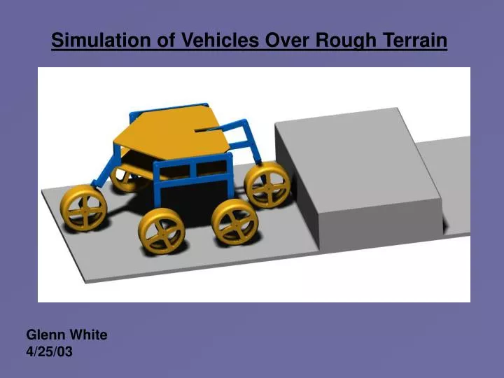
Simulation of Vehicles Over Rough Terrain Glenn White 4/25/03
Contents • Challenge of rough terrain to vehicle design • The Shrimp: A passive design prototype • Methods of analyzing the performance of vehicles • IV. Building a virtual prototype • V. Shrimp front 4-bar design • Surface contacts in Visual Nastran • Conclusion
I. The Challenges of Rough Terrain to Vehicle Design • Vehicle must be able to operate on a variety of different surfaces • Hard, soft, sand, rock, wet, dry, etc. • Vehicle must maintain stability over obstacles • Unpredictable surface profile • Unknown bump size • Two different methods to design for stability • Passive: Uses passive components such as springs, dampers, levers, and 4-bars to achieve stability • Active: Uses electronic components such as sensors and actuators to maintain stability
II. The Shrimp: A Passive Design Prototype • Uses 4-bars, springs, and dampers as main passive components • The only actuators are motors used to drive the wheels • Created by the Institut de Systèmes Robotiques and BlueRobotics • http://dmtwww.epfl.ch/isr/asl/systems/shrimp.html • http://www.bluebotics.com/products/shrimp/
III. Different Methods of Analyzing Vehicle Performance • Physical Prototyping • Advantages: • -Represents the actual performance of the vehicle by gathering real data on different obstacles and surface conditions • Disadvantages: • -Expensive • -Time consuming • -Hard to modify or change vehicle parameters • Virtual Prototyping • Advantages: • -Can easily change sizes, masses, inertias, spring rates, etc. • -Quick, inexpensive • Disadvantages: • -Requires large amounts of computing time • -True representations of obstacles and surface conditions are not easily modeled
IV. The Steps for Building a Virtual Prototype in • Solid Works and Visual Nastran • Determine design and dimensions • Model individual parts and assemble in Solid Works • Export the Solid Works file to Visual Nastran • Set up the constraints and simulation settings • Run simulation
Determine Design and Dimensions Dimensions are in (mm)
Model Individual Parts and Assemble in Solid Works Solid Works Final Assembly
Suggestions for Creating Assembly in Solid Works • Assemble project in the exact orientation that you want it to appear in • Visual Nastran. It is difficult to adjust the position of components • accurately from inside Visual Nastran. • Model parts so that they can be easily changed • For example: In the 4-bar link shown below, the driving dimension for the length is the distance between the revolute joints and not the total length of the link. Link Driving Dimensions
Suggestions Continued: • Mate revolute joints by selecting concentric surfaces on the two parts • This indicates to Visual Nastran that the joint should be revolute Mate these surfaces
Export Solid Works File to Visual Nastran Rigid Joint Revolute Joint Revolute Motor View with all constrains visible Spring View with constrains hidden
Suggestions for Simulation in Visual Nastran • Use “point contact” surface detection instead of “faceted” surface • detection for rolling contacts like wheel • Implement this by modeling both “spherical” and “cylindrical” • wheels and assembling both in model • Set only the spherical wheels to contact and then hide them Cylindrical Wheel Spherical Wheel
V. The Importance of the Front 4-Bar Design • This is the main passive component that the Shrimp utilizes • The Shrimp performance over different obstacles is highly • dependant on the configuration of the 4-Bar. The two most • important considerations are: • 1. The location of the instant center of the coupler link • This determines the initial motion of the 4-bar and the • direction of force that helps the 4-bar move as it encounters • an obstacle • 2. The migration of the instant center as the 4-bar moves • This determines the change in motion and force that the 4- • bar experiences
Two Different 4-Bar Designs and Locations of Instant Centers Front 4-bar Instant center behind and below (original design) Instant center in front and above (modified design)
Wheel Paths of the Two Different Designs • The modified design is better suited to absorbing obstacles by • moving up and away from the obstacle Initial Position Initial Position Modified Design Original Design
The Migration of the Instant Centers Original Design Modified Design
Simulation of the Two Designs • The obstacle is a vertical wall • All other parameters are equal • Zero spring force Modified Design Original Design
Conclusions from the Design Comparison • The wheel path of the modified design is better suited to absorbing • obstacles -The wheel moves up and away from the obstacle, thus absorbing the frontal impact, however small. This allows the wheel a larger amount of time to move up and over the obstacle without greatly effecting the velocity of the rest of the shrimp. • The original design moves in a more vertical path and does not allow the obstacle to be absorbed. Therefore, the velocity of the entire shrimp is adversely affected. • The location and migration of the instant center in the modified • design is beneficial to overcoming obstacles • -The instant centers lie either in front and above the wheel or behind and below the wheel. Therefore, a beneficial upward force is created when encountering obstacles, even when the obstacle imparts a horizontal force on the wheel.
VI.Simulation of Surface Contacts in Visual Nastran • Two different types of surface contact detection: • Point contact • Used for objects that have a single point contact, like a sphere on a plane • Advantages • Fast • Simple • Accurate • Faceted surface contact • Used to model non-spherical objects, like a cylinder or cube on a plane • Works by breaking the object up into many facets (flat surfaces) depending on the precision required • Example: A circle would be approximated by an n-sided polygon
Facets Continued: • Two models of faceted surface contact in Visual Nastran: • Penetration • Allows objects to penetrate each other a very small amount • This method is quicker, but less accurate • No penetration • Does not allow objects to penetrate each other • This method is slower, but more accurate
Study: A Comparison of Different Surface Contact Methods • Purpose: To identify the differences between the contact methods • Method: • Roll disks of equal mass and inertia down an inclined plane • Vary the time step and contact method • Obtain linear and angular displacement for simulation time of 0.5 sec • Calculate theoretical results and compare • Given: • m = 0.025 kg • I = 0.795 kg-mm² • Number of facets Disk 1 = 86; Disk 2 = 172; Disk 3 = 344 • Sphere has same mass and inertia properties • Angle of inclined plane = 10° • Simulation time = 0.5 sec
Study: Simulation Setup: Example Visual Nastran simulation 344 Facets 172 Facets 86 Facets Sphere • Ran simulations for all contact methods and the following time steps: • dt = .005, .0025, .00125, .000625, .0003125, .00015625
Study: Data Data Output: Example data output from Visual Nastran Wheel 1 Wheel 2 Wheel 3 Facets = 86 Facets = 172 Facets = 344 Angular Displacement Linear Displacement Note: By right clicking on the graphical data output, you can change it to numerical output
Study: Data • Observations from the Simulation: • Graphs of linear displacement contain no errors in the time step region • considered • Graphs of angular displacement contain errors due to slip • These errors decrease as the number of facets and step size is decreased • Point contact graphs contain no error in this time step region
Study: Results • Observations from the results: • Faceted Simulation • Precision of simulation increases with increasing number of facets and • decreasing time step • No penetration is more precise than penetration • Error in penetration model ranged from 7% to 36% • Error in no penetration model ranged from 7% to 27% • Point Contact Simulation • Precision of simulation increases with decreasing time step • Error in this model was less than 0.05% for all time step sizes considered
VII. Conclusion • Analyzing rough terrain vehicle behavior can be time consuming and expensive • Example of the shrimp • Two methods for analysis: • Physical Prototype: Accurate behavior, but difficult to change parameters • Virtual Prototype: Approximate behavior, but easy to change parameters • Virtual prototyping allows us to study aspects of the shrimp, like the front 4-bar, quickly and easily • This revealed that the location and path of the instant center migration is very important in determining the forces on the 4-bar and the way it moves • Virtual prototyping, however, is limited by the effectiveness of the mathematical model and the computing time necessary to solve the model. There is a trade off between time step and accuracy.