Download
1 / 16
160 likes | 312 Views
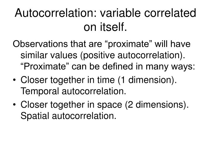
Autocorrelation: variable correlated on itself. Observations that are “proximate” will have similar values (positive autocorrelation). “Proximate” can be defined in many ways: Closer together in time (1 dimension). Temporal autocorrelation.

E N D
Autocorrelation: variable correlated on itself. Observations that are “proximate” will have similar values (positive autocorrelation). “Proximate” can be defined in many ways: • Closer together in time (1 dimension). Temporal autocorrelation. • Closer together in space (2 dimensions). Spatial autocorrelation.
Degree of autocorrelation can be calculated: • For dependent or independent variables. • For regression residuals.
Autocorrelation of regression residuals creates problem. • Usual view: estimated coefficients are unbiased, but standard errors are biased. • Alternative view: autocorrelated residuals signal presence of omitted variables. estimated coefficients are biased.
Residuals: Hedonic House Price Model (Blue paid too little; Red paid too much)
12 Proximity Matrices • Physical Distance • Language Phylogeny • Religion • Huntington Civlization • Colonial/Imperial • Level of Development • Ecology • Trade • Formal Treaty • Allies • Enemies • Event Frequency
The 12 selected languages are on the periphery of the digraph. Links point toward higher taxonomic levels, with all nodes ultimately connected to the node labeled Indo-European. The numbers indicate for selected nodes the maximum path length leading to that node. The taxonomy is from Grimes 2000