Download
1 / 24
250 likes | 532 Views
Professor Walter W. Olson Department of Mechanical, Industrial and Manufacturing Engineering University of Toledo. Modeling. Outline of Today’s Lecture. Review Feedback Open Loop Systems Closed Loop System Positive Feedback Negative Feedback Basic Control actions Models Dynamics

E N D
Professor Walter W. Olson Department of Mechanical, Industrial and Manufacturing Engineering University of Toledo Modeling
Outline of Today’s Lecture • Review • Feedback • Open Loop Systems • Closed Loop System • Positive Feedback • Negative Feedback • Basic Control actions • Models • Dynamics • States • Phase Plots • Example: Predator Prey Model
Open Loop Control • Usually “set point” systems • Advantages • Simple • Insensitive to environment • Set and forget • Disadvantages • Non correcting • Sensitive to disturbances • Insensitive to environment • Examples • Irrigation systems • Washing machines Sensing Compute Actuate
Closed Loop Control Actuate Sense • Adds a feedback loop to the control system • For computational purposes, it is shown as Controller Plant Compute Sensor Disturbance + or - + or - Output Input + or - + or -
Positive Feedback Background sound + + Sound Ambient Sound + + + + Controller Controller Plant Plant + + Speaker Amplifier Previous Vibrations Sensor Sensor Guitar String w/ pickup Plucked String String Vibrations 2 possible models Vibrating Guitar String Amplifier Speaker Magnetic Pickup Positive Feedback Clip
Positive Feedback • Positive feedback is used to increase the actuation in the loop. • Advantages • Increased results • Faster results • Finds extremes • (maxima and minima) • Disadvantages • Consumes energy • Subject to local extremes (introns) • May become unstable • May destroy system • Examples: • Metal finders • Searches • Stock market programs • Genetic Algorithm performance measure build population test Worst Best Culled from Population create mutations Results
Negative Feedback Error Signal Disturbance + + + Controller Controller Plant Plant Output - Input Sensor Sensor Salt Desired Heart Beat + + + Heart Beat - Parasympathetic/Sympathetic System Heart homeostasis Nerves
Negative Feedback • Negative Feedback is used to reduce error • Advantages • Controls to a set point • Robustness to disturbances (uncertainty) • Rejection of distortion • Disadvantages • Prone to oscillation • Instability • Complexity • Coupling • Examples • Set point control • Tracking • Chang the system dynamics
Basic Control Actions • Bang-Bang (Off-On) • Fixed two state or multistate control actions • Control question: how to chose? • Proportional • Control in proportion to error • Integral • Control based on size and duration of error • Derivative • Control based on size and change of error • Combined (PID) • All three: Proportional, Integral and Derivative • Most used
Models • A model is a representation of something • The something can be an idea, a concrete object or an abstract object • It is NOT the real thing: they are simplifications • it is a fiction of our imagination • Models can take many forms • Solid • Blocks • Equations • Computer programs • Word descriptions • Symbols
Models • It is NOT the real thing: they are simplifications • it is a fiction of our imagination • Models are used for • visualization • understanding • explaining to others • analysis • predict • improve • The value of amodel is howwell it servesthe purposeused for
Models • Different models answer different questions • As a model developer, you need to chose the right model for your problem How will costs change with the strength of the landing gear? How much vertical force is the landing gear putting on the nose? How high should the tire pressure be? At what point can the pilot rotate the aircraft to take weight off the nose wheel? How much heat is built up in the tire on a takeoff roll?
Dynamics • defn (TheFreeDictionary): The branch of mechanics that is concerned with the effects of forces on the motion of a body or system of bodies, especially of forces that do not originate within the system itself. Also called kinetics. • Things move! • If we are to control movement we need to know how they move
Dynamics • Models of dynamics used in this course: • Based on functions of time • Differential equations • time is considered continuous • Difference equations • time is considered discrete
State • A state is a set of variables whose values when known completely define the dynamics (motion) • State variables for nose wheel example: • The parameters of the example are • So, what about ?
State • So, what about ? • These are completely determined by the statevariables! • We can rewrite the equations as
Phase Plot • A phase plot is a plot of a state variable vs. another state variable • Useful in understanding how the dynamics change with changes in state • To see how the dynamics are represented by the phase plot, consider the predator prey problem • we will first use differential equationsthen difference equations
Predator Prey Model • Volterra – Lotke model • Vito Volterra and Alfred J. Lotke independently developed this useful model • Explains the growth of a thing that depends on the growth of another thing • Lynx and hares or whales and krill are typically used to demonstrate the model but it could be two infantry units fighting each other or two stock firms trying to acquire the same limited commodity • Let x(t) represent the prey (hares, krill, xthInf, etc.) and y(t) represent the predator (lynx, whales, nth Inf, etc.) • Prey population growth rate without predators is assumed proportional to population size But….
Predator Prey Model • But there are predators! • The predators [eat, destroy, acquire…] the prey in proportion to the number of prey and predators. • The predator population without sufficient prey dies out at a rate of • But there are predators that are [eaten, destroyed, acquired …] that sustain the predators in proportion to both populations sizes:
Predator Prey Model • The model is • subject to • x(t) = prey population size • y(t) = predator population size • a = growth rate of prey • b = rate of prey predation • m = death rate of predators • n = rate of predator sustenance • Model Solution • State Variables: x, y • Note the controls in this nonlinear, coupled, model
Predator Prey Model • Lynx – Hare ( data from Leigh, 1968) • Continuous Model
Discrete Predator Prey Model • To discretize, • choose time step, h • replace • The difference equations are • If h = 1 year, the model is • Evaluation: • with x(0)=80, y(0)=30 • a = 0.7, b = 0.03, • m=0.99, n = 0.03 • Initially h = 1 year
Discrete Predator Prey Model • Choice of time step • is critical to • discrete modeling • Unstable Model! • Problem: the time step is too big! • with h = 0.1 years • The smaller the time step, the more • accurate the model but more computations
Summary • We discussed modeling • Models are simplifications • Dynamics: things move! • differential equations • difference equations • States • a set of variables whose values when known completely define the dynamics (motion) • Phase Plots • a plot of a state variable vs. another state variable • Example: Predator Prey Model • Next: State Space Models