Download
1 / 78
780 likes | 920 Views
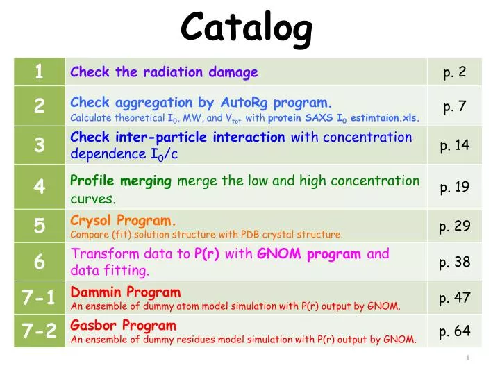
Catalog. 1. Check the radiation damage. 1. Import multiple ACSII of output files of each frame and combined data. 2. Plot all curves in a graph. 3. Check the low-q region in the all profiles. If all profiles are overlapped well at low-q region, no radiation damage occurs .

E N D
1. Import multiple ACSII of output files of each frame and combined data
If all profiles are overlapped well at low-q region, no radiation damage occurs.
2. Check aggregation by AutoRg program. Calculate theoretical I0, MW, and Vtotwith protein SAXS I0 estimtaion.xls.
4. In Guinier tab, check the aggregation and define the qmin before unreliable range.
5. In Info tab, read the sRg limits (Guinier region), I0, and Rgvalues.
One can calculate theoretical MW, I0, and Vtotwith protein SAXS I0 estimtaion.xls. (spreadsheet edited by Dr. Jeng) 1 3 4 2 5 6
3. Check inter-particle interaction with concentration dependence I0/c
1. Import multiple ACSII of all different concentration curves.
4. Confirm if concentration dependence is distinguishable at low-q region.
4. Profile merging merge the low and high concentration curves.
2. Click “Tools” to select the low and high concentration data for merging.
4. Input the parameters into nBeg (begin point #) and nEnd (end point #) of Data Processing.
4-2. Remove the points of inter-particle interference region and divergence region
6. Fine tune the eEnd point to make sure that the endpoints are superimposed with the merged curve.
5. Crysol Program Compare (fit) solution structure with PDB crystal structure.
3. Maximum order of harmonics <15>: Order of Fibonacci grid <17>: Maximum s value <0.5>: Number of points <51>: Account for explicit hydrogens <no>: Fit the experimental curve <yes>:
5. Subtract constant <no>: Angular units in the input file <1>: Electron density of the solvent <0.334>: Plot the fit <yes>: Another set of parameters <no>: Press “ ” to terminate the program
6. Plot the 1st (experimental scattering vector) and 2nd (theoretical intensity in solution) columns of fit file. fitted solution envelope of native cyt. c
7. Open the log file to read the experimental and theoretical Rg values.
6. Transform data to P(r) with GNOM program and data fitting.
3. • No of start points to skip [ 0 ] : • Input data, second file [ none ] : • No of end points to omit [ 0 ] : • Angular scale (1/2/3/4) [ 1 ] : • Plot input data (Y/N) [ Yes ] :
4. • File containing expert parameters [ none ] : • Kernel already calculated (Y/N) [ No ] : • Type of system (0/1/2/3/4/5/6) [ 0 ] : • Zero condition at r=rmin (Y/N) [ Yes ] : • Zero condition at r=rmax (Y/N) [ Yes ] :
6. • Number of points in real space [ 101 ] : • Kernel-storage file name [ kern.bin ] : • Experimental setup (0/1/2) [ 0 ] : • Initial ALPHA [ 0.0 ] :
7-1. DamminProgram An ensemble of dummy atom model simulation with P(r) output by GNOM.
1. Select the Mode: <[F]>ast, [S]low, [J]ag, [K]eep, [E]xpert < Fast >: