Download
1 / 40
450 likes | 688 Views
Hybrid Monte-Carlo simulations of electronic properties of graphene [ ArXiv:1206.0619]. P. V. Buividovich ( Regensburg University). Graphene ABC. Graphene : 2D carbon crystal with hexagonal lattice a = 0.142 nm – Lattice spacing π orbitals are valence orbitals (1 electron per atom)

E N D
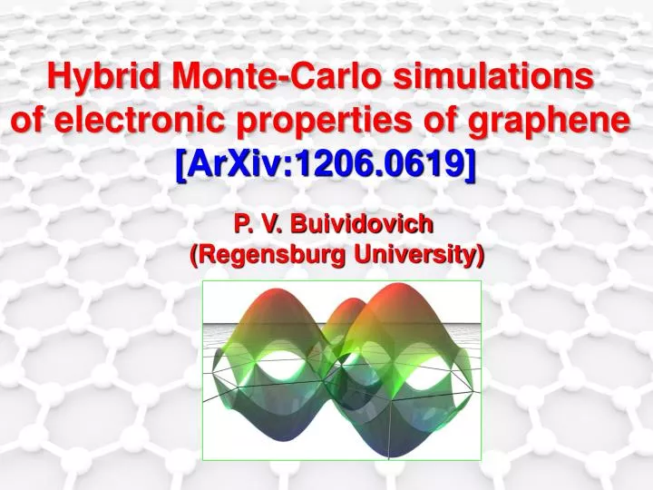
Hybrid Monte-Carlo simulations of electronic properties of graphene [ArXiv:1206.0619] P. V. Buividovich (Regensburg University)
Graphene ABC • Graphene: 2D carbon crystal with hexagonal lattice • a = 0.142 nm – Lattice spacing • π orbitals are valence orbitals (1 electron per atom) • Binding energy κ ~ 2.7 eV • σ orbitals create chemical bonds
Geometry of hexagonal lattice Two simple rhombic sublattices А and В Periodic boundary conditions on the Euclidean torus:
The “Tight-binding” Hamiltonian Fermi statistics “Staggered” potential m distinguishes even/odd lattice sites
Physical implementation of staggered potential Graphene Boron Nitride
Spectrum of quasiparticles in graphene Consider the non-Interacting tight-binding model !!! One-particle Hamiltonian Eigenmodes are just the plain waves: Eigenvalues:
Spectrum of quasiparticles in graphene Close to the «Dirac points»: “Staggered potential” m = Dirac mass
Spectrum of quasiparticles in graphene Dirac points are only covered by discrete lattice momenta if the lattice size is a multiple of three
Symmetries of the free Hamiltonian 2 Fermi-points Х 2 sublattices = 4 components of the Dirac spinor Chiral U(4) symmetry (massless fermions): rightleft Discrete Z2 symmetry between sublattices АВ U(1) x U(1) symmetry: conservation of currents with different spins
Particles and holes • Each lattice site can be occupied by two electrons (with opposite spin) • The ground states is electrically neutral • One electron (for instance ) • at each lattice site • «Dirac Sea»: • hole = • absence of electron • in the state
Lattice QFT of Graphene Redefined creation/ annihilation operators Charge operator Standard QFT vacuum
Electromagnetic interactions Link variables (Peierls Substitution) Conjugate momenta = Electric field Lattice Hamiltonian (Electric part)
Electrostatic interactions Effective Coulomb coupling constant α ~ 1/137 1/vF ~ 2 (vF~ 1/300) Strongly coupled theory!!! Magnetic+retardation effects suppressed • Dielectric permittivity: • Suspended graphene • ε = 1.0 • Silicon DioxideSiO2 • ε ~ 3.9 • Silicon CarbideSiC • ε ~ 10.0
Electrostatic interactions on the lattice Discretization of Laplacian on the hexagonal lattice reproduces Coulomb potential with a good precision
Main problem: the spectrum of excitations in interacting graphene Lattice simulations, Schwinger-Dyson equations ??? Renormalization, LargeN, Experiment [Manchester group, 2012] Spontaneous breaking of sublattice symmetry = mass gap = condensate formation = = decrease of conductivity
Numerical simulations: Path integral representation Technical details Decomposition of identity Eigenstates of the gauge field Fermionic coherent states (η – Grassman variables) Gauss law constraint (projector on physical space)
Numerical simulations: Path integral representation Technical details • Electrostatic potential field • Lagrange multiplier for the Gauss’ law • Analogue of the Hubbard-Stratonovich field :
Numerical simulations: Path integral representation Technical details Lattice action for fermions (no doubling!!!): Path integral weight: Positive weight due to two spin components!
Hybrid Monte-Carlo: a brief introduction Problem: generate field configurations φ(x) with probability For graphene– nonlocal action due to fermion determinant Metropolis algorithm • Propose new field • configurations with probability • Accept/reject with probability • Exact algorithm • Local updates of fields • BUT: • Fermion determinant recalculation
Hybrid Monte-Carlo: a brief introduction Molecular Dynamics Classical motion with If ergodic: π(x) – conjugate momentum for φ(x) • Global updates of fields ϕ(x) • 100% acceptance rate • BUT: • Energy non-conservation for numerical integrators
Hybrid Monte-Carlo = Molecular Dynamics + Metropolis • Use numerically integrated Molecular Dynamics trajectories as Metropolis proposals • Numerical error is corrected by accept/reject • Exact algorithm • Ψ-algorithm [Technical]: • Represent determinant • as Gaussian integral Molecular Dynamics Trajectories
Numerical simulations using the Hybrid Monte-Carlo method • Hexagonal lattice • Noncompact U(1) gauge field • Fast heatbath algorithm outside of graphene plane • Geometry: graphene on the substrate
Breaking of lattice symmetry Intuition from relativistic QFTs (QCD): Symmetry breaking = = gap in the spectrum • Anti-ferromagnetic state • (Gordon-Semenoff 2011) • Kekule dislocations • (Araki 2012) • Point defects
Spontaneous sublattice symmetry breaking in graphene Order parameter: The difference between the number of particles on А and Вsublattices ΔN = NA – NB “Mesons”: particle-hole bound state
Differences of particle numbers on lattices of different size Extrapolation to zero mass
Susceptibility of particle number differences
Conductivity of graphene Current operator: = charge, flowing through lattice links Retarded propagator and conductivity:
Conductivity of graphene: Green-Kubo relations Technical details Current-current correlators in Euclidean space: Green-Kubo relations: Thermal integral kernel:
Conductivity of graphene Technical details σ(ω) – dimensionless quantity (in a natural system of units), in SI: ~ e2/h Conductivity from Euclidean correlator: an ill-posed problem Maximal Entropy Method Approximate calculation ofσ(0): AC conductivity, averaged overw ≤ kT
Conductivity of graphene: free theory For small frequencies (Dirac limit): Threshold value w = 2 m Universal limiting value atκ>> w >> m: σ0 = π e2/2 h=1/4 e2/ħ Atw = 2 m: σ = 2 σ0
Conductivity of graphene: Free theory
Current-current correlators: numerical results κΔτ=0.15, m Δτ = 0.01, κ/(kT) = 18, Ls = 24
Conductivity of grapheneσ(0): numerical results (approximate definition)
Direct measurements of the density of states • Experimentally motivated definition • Valid for non-interacting fermions • Finite μ is introduced in observables only (partial quenching)
Conclusions • Electronic properties of graphene at half-filling can be studied using the Hybrid Monte-Carlo algorithm. • Sign problem is absent due to the symmetries of the model. • Signatures of insulator-semimetal phase transition for monolayer graphene. • Order parameter: • difference of particle numbers on two simple sublattices • Spontaneous breaking of sublattice symmetry is accompanied by a decrease of conductivity • Direct measurements of the density of states indicate increasing Fermi velocity • see ArXiv:1206.0619
Outlook • Lattice simulations by independent groups: • Spontaneous symmetry breaking in graphene • at α ~ 1 (ε ~ 4 – SiO2) • [Drut, Lahde; Hands; Rebbi; ITEP Group; PB] • Experimentally: suspended graphene is conducting, no signature of a gap in the spectrum [Elias et al. 2011] • What are we missing? Mass? Finite volume? • Our strategy works not so well as for Lattice QCD • Another interesting case: double-layered graphene,