Download
1 / 46
460 likes | 816 Views
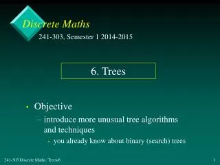
Discrete Maths. 242-213 , Semester 2, 2013-2014. Objective introduce more unusual tree algorithms and techniques you already know about binary (search) trees. 12 . Trees. Overview. Uses of Trees (Rooted) Tree Terminology Spanning Trees Minimal Spanning Trees More Information.

E N D
Discrete Maths 242-213, Semester 2, 2013-2014 • Objective • introduce more unusual tree algorithms and techniques • you already know about binary (search) trees 12. Trees
Overview • Uses of Trees • (Rooted) Tree Terminology • Spanning Trees • Minimal Spanning Trees • More Information
1. Uses of Trees Davenport S. Williams S. Williams S. Williams Bartoli V. Williams V. Williams Wimbledon Womens Tennis
Organizational Chart President Vice-President for Academics Vice-President for Admin. Dean of Engineering Dean of Business Planning Officer Purchases Officer . . . . . . . . Head of CoE Head of EE Head of AC. . . . .
Saturated Hydrocarbons H H H H • Non-rooted (free) trees • a free tree is a graph with no cycles C H H C C C H H C H H H C H H H C H H Isobutane H C H H Butane H
A Computer File System / usr bin tmp bin ad spool ls mail who junk ed vi exs opr uucp printer
2. (Rooted) Tree Terminology • e.g. Part of the ancient Greek god family: levels 0 Uranus 1 Aphrodite Kronos Atlas Prometheus 2 Eros Zeus Poseidon Hades Ares 3 Apollo Athena Hermes Heracles : :
Some Definitions • Let T be a tree with root v0. • Suppose that x, y, z are verticies in T. • (v0, v1,..., vn) is a simple path in T (no loops). • a) vn-1 is the parent of vn. • b) v0, ..., vn-1 are ancestors of vn • c) vn is a child of vn-1 continued
d) If x is an ancestor of y, then y is a descendant of x. • e) If x and y are children of z, then x and y are siblings. • f) If x has no children, then x is a terminal vertex (or a leaf). • g) If x is not a terminal vertex, then x is an internal (or branch) vertex. continued
h) The subtree of T rooted at x is the graph with vertex set V and edge set E • V contains x and all the descendents of x • E = {e | e is an edge on a simple path from x to some vertex in V} • i) The length of a path is the number of edges it uses, not verticies. continued
j) The level of a vertex x is the length of the simple path from the root to x. • k) The height of a vertex x is the length of the simple path from x to the farthest leaf • the height of a tree is the height of its root • l) A tree where every internal vertex has exactly m children is called a full m-ary tree.
Applied to the Example • The root is Uranus. • A simple path is {Uranus, Aphrodite, Eros} • The parent of Eros is Aphrodite. • The ancestors of Hermes are Zeus, Kronos, and Uranus. • The children of Zeus are Apollo, Athena, Hermes, and Heracles. continued
The descendants of Kronos are Zeus, Poseidon, Hades, Ares, Apollo, Athena, Hermes, and Heracles. • The leaves (terminal verticies) are Eros, Apollo, Athena, Hermes, Heracles, Poseidon, Hades, Ares, Atlas, and Prometheus. • The branches (internal verticies) are Uranus, Aphrodite, Kronos, and Zeus. continued
The subtree rooted at Kronos: Kronos Zeus Poseidon Hades Ares Apollo Athena Hermes Heracles continued
The length of the path {Uranus, Aphrodite, Eros} is 2 (not 3). • The level of Ares is 2. • The height of the tree is 3.
3. Spanning Trees • A spanning tree T is a subgraph of a graph G which contains all the verticies of G. • Example graph G: a b c d e f h g continued
One possible spanning tree: a b the tree is drawn with thick lines c d e f h g
3.1. Example: IP Multicasting • A network of computers and routers: source computer router continued
How can a packet (message) be sent from the source computer to every other computer? • The inefficient way is to use broadcasting • send a copy along every link, and have each router do the same • each router and computer will receive many copies of the same packet • loops may mean the packet never disappears! continued
IP multicasting is an efficient solution • send a single packet to one router • have the router send it to 1 or more routers in such a way that a computer never receives the packet more than once • This behaviour can be represented by a spanning tree. continued
The spanning tree for the network: source computer the tree is drawn with thick lines router
3.2. Finding a Spanning Tree • There are two main types of algorithms: • breadth-first search • depth-first search
3.3. Breadth-first Search • Process all the verticies at a given level before moving to the next level. • Example graph G (again): a b c d e f h g
Informal Algorithm • 1) Put the verticies into an ordering • e.g. {a, b, c, d, e, f, g, h} • 2) Select a vertex, add it to the spanning tree T: e.g. a • 3) Add to T all edges (a,X) and X verticies that do not create a cycle in T • i.e. (a,b), (a,c), (a,g) T = {a, b, c, g} a g b c continued
a level 1 g b c • Repeat step 3 on the verticies just added, these are on level 1 • i.e. b: add (b,d) c: add (c,e) g: nothing T = {a,b,c,d,e} • Repeat step 3 on the verticies just added, these are on level 2 • i.e. d: add (d,f) e: nothing T = {a,b,c,d,e,f} d e a g b c level 2 d e f continued
a • Repeat step 3 on the verticies just added, these are on level 3 • i.e. f: add (f,h) T = {a,b,c,d,e,f,h} • Repeat step 3 on the verticies just added, these are on level 4 • i.e. h: nothing, so stop g b c d e level 3 f h continued
Resulting spanning tree: a b a different spanning tree from the earlier solution c d e f h g
3.4. Depth-first Search • Process all the verticies down one path, then backtrack (go back) to verticies along other paths. • Example graph G (again): a b c d e f h g
Informal Algorithm • 1) Put the verticies into an ordering • e.g. {a, b, c, d, e, f, g, h} • 2) Select a vertex, add it to the spanning tree T: e.g. a • 3) Add the edge (a,X) where X is the smallest vertex in the ordering, and does not make a cycle in T • i.e. (a,b), T = {a, b} a b continued
a b d • 4) Repeat step 3 with the new vertex, until there is no possible new vertex • i.e. add the edges (b,d) (d,c) (c,e) (e,f) (f,h) T = {a,b,d,c,e,f,h} • 5) At this point, there is no (h,X), so backtrack to a vertex that does have another edge: • parent of h == fbut there is no new (f,X) to add, so backtrack c e f h continued
a b • parent of f == e • there is an (e,g) to add, so repeat step 3 with e • 6) After g is added, there are no further verticies to add, so stop. d c e g f h continued
Resulting spanning tree: a a different spanning tree from the breadth-first solution b c d e f h g
4. Minimal Spanning Tree • A minimal spanning tree T is a subgraph of a weighted graph G which contains all the verticies of G and whose edges have the minimum summed weight. • Example weighted graph G: A 4 B 5 3 2 C D 1 6 3 6 E 2 F
A 4 B • A minimal spanning tree (weight = 12): • A non-minimal spanning tree (weight = 20): 5 3 2 C D 1 6 3 6 E 2 F A 4 B 5 3 2 C D 1 6 3 6 E 2 F
4.1. Prim's Algorithm • Prim's algorithm finds a minimal spanning tree T by iteratively adding edges to T. • At each iteration, a minimum-weight edge is added that does not create a cycle in the current T. Robert Clay Prim (1921 – )
A 4 B Informal Algorithm 5 3 2 C D 1 6 3 6 • For the graph G. • 1) Add any vertex to T • e.g A, T = {A} • 2) Examine all the edges leaving {A} and add the vertex with the smallest weight. • edge weight(A,B) 4(A,C) 2(A,E) 3 • add edge (A,C), T becomes {A,C} E 2 F continued
3) Examine all the edges leaving {A,C} and add the vertex with the smallest weight. • edge weight edge weight(A,B) 4 (C,D) 1(A,E) 3 (C,E) 6(C,F) 3 • add edge (C,D), T becomes {A,C,D} continued
4) Examine all the edges leaving {A,C,D} and add the vertex with the smallest weight. • edge weight edge weight(A,B) 4 (D,B) 5(A,E) 3 (C,E) 6(C,F) 3 (D,F) 6 • add edge (A,E) or (C,F), it does not matter • add edge (A,E), T becomes {A,C,D,E} continued
5) Examine all the edges leaving {A,C,D,E} and add the vertex with the smallest weight. • edge weight edge weight(A,B) 4 (D,B) 5(C,F) 3 (D,F) 6(E,F) 2 • add edge (E,F), T becomes {A,C,D,E,F} continued
6) Examine all the edges leaving {A,C,D,E,F} and add the vertex with the smallest weight. • edge weight edge weight(A,B) 4 (D,B) 5 • add edge (A,B), T becomes {A,B,C,D,E,F} • All the verticies of G are now in T, so we stop. continued
Resulting minimum spanning tree (weight = 12): A 4 B 5 3 2 C D 1 6 3 6 E 2 F
4.2. Kruskal's Minimum Spanning Tree Algorithm • At the start, the minimum spanning tree T consists of all the verticies of the weighted graph G, but no edges. • At each iteration, add an edge e to T having minimum weight that does not create a cycle in T. • When T has n-1 edges, stop. Joseph Bernard Kruskal (1928 – 2010)
Example iter edge 1 (c,d) 2 (k,l) 3 (b,f) 4 (c,g) 5 (a,b) 6 (f, j) 7 (b,c) 8 (j,k) 9 (g,h) 10 (i, j) 11 (a,e) • Graph G: b c d a 2 3 1 2 3 1 3 g f h e 4 3 3 4 4 2 3 i l j 3 3 k 1 continued
Minimum spanning tree (weight = 24): b c d a 2 3 1 2 3 1 3 g f h e 4 3 3 4 4 2 3 i l j 3 3 k 1
4.3. Difference between Prim and Kruskal • Prim's algorithm chooses an edge that must already be connected to a vertex in the minimum spanning tree T. • Kruskal's algorithm can choose an edge that may not already be connected to a vertex in T.
5. More Information • Discrete Mathematics and its ApplicationsKenneth H. RosenMcGraw Hill, 2007, 7th edition • chapter 11, sections 11.1, 11.4, 11.5