Download
1 / 73
730 likes | 879 Views
Course Name: Systems Biology I Conducted by- Shigehiko kanaya & Md. Altaf-Ul-Amin. Dates of Lectures: April: 8, 15, 22 May: 13, 20, 27 June: 3 Lecture Time: Tuesdays 9:20-10:50 Website http://kanaya.naist.jp/Lecture/. Syllabus

E N D
Course Name: Systems Biology I Conducted by- Shigehiko kanaya & Md. Altaf-Ul-Amin
Dates of Lectures: April: 8, 15, 22 May: 13, 20, 27 June: 3 Lecture Time: Tuesdays 9:20-10:50 Website http://kanaya.naist.jp/Lecture/
Syllabus Introduction to Graphs/Networks, Different network models, Properties of Protein-Protein Interaction Networks, Different centrality measures Protein Function prediction using network concepts, Application of network concepts in DNA sequencing, Line graphs Concept and types of metric, Hierarchical Clustering, Finding clusters in undirected simple graphs: application to protein complex detection Introduction to KNApSAcK database, Metabolic Reaction system as ordinary differential equations, Metabolic Reaction system as stochastic process Metabolic network and stoichiometric matrix, Information contained in stoichiometric matrix, Elementary flux modes and extreme pathways Graph spectral analysis/Graph spectral clustering and its application to metabolic networks Normalization procedures for gene expression data, Tests for differential expression of genes, Multiple testing and FDR, Reverse Engineering of genetic networks Finding Biclusters in Bipartite Graphs, Properties of transcriptional/gene regulatory networks, Introduction to software package Expander Introduction to signaling pathways, Selected biological processes: Glycolytic oscillations, Sustained oscillation in signaling cascades
The crowded Environment inside the cell Some of the physical characteristics are as follows: Viscosity > 100 × μ H20 Osmotic pressure < 150 atm Electrical gradient ~300000 V/cm Near crystalline state The osmotic pressure of ocean water is about 27 atm and that of blood is 7.7 atm at 25oC Without a complicated regulatory system all the processes inside the cell cannot be controlled properly. Source: Systems biology by Bernhard O. Palsson
From Genome to Phenome (Dynamic) Phenotype X Phenome Metabolites (Bio-chemical molecules) Metabolome Proteins-Amino Acid Sequences Proteome mRNA and other RNAs - Nucleotide sequence-Single Stranded Transcriptome DNA –Nucleotide sequence- ATCTGAT……Double Helix Genome (Gene set) (Statiic) Progressing genome projects: many kinds of “–omics” works have progressed such as genomics, transcriptomics, proteomics, metabolomics …. These are dynamic information reflecting to Phenome.
Integration of omics to define elements (genome, mRNAs, Proteins, metabolites) Understanding organism as a system (Systems Biology) Understanding species-species relations (Survival Strategy) Bioinofomatics Genome: 5’ 3’ b c h i k m 3’ 5’ a d e f g j l Transcriptome: Activation (+) A 5’ 3’ b c h i k m 3’ 5’ G a d e f g j l Repression (-) G Proteome, Interactome Protein A B C D E F G H I J K L M Function Unit A B C D E G H K I L M J F Metabolome FT-MS comprehensive and global analysis of diverse metabolites produced in cells and organisms B C I L Metabolite 1 Metabolite 2 Metabolite 3 Metabolite 5 D E F Metabolic Pathway H K Metabolite 4 Metabolite 6
Introduction to Graphs/NetworksRepresenting as a network often helps to understand a system
Konigsberg bridge problem Konigsberg was a city in present day Germany encompassing two islands and the banks of Pregel River. The city was connected by 7 bridges. Problem: Start at any point, walk over each bridge exactly once and return to the same point. Possible?
Konigsberg bridge problem Konigsberg was a city in present day Germany including two islands and the banks of Pregel River. The city was connected by 7 bridges. Problem: Start at any point, walk over each bridge exactly once and return to the same point. Possible?
Konigsberg bridge problem Konigsberg was a city in present day Germany including two islands and the banks of Pregel River. The city was connected by 7 bridges. Problem: Start at any point, walk over each bridge exactly once and return to the same point. Possible?
Konigsberg bridge problem Problem: Start at any point, walk over each bridge exactly once and return to the same point. Possible? This problem was solved by Leonhard Eular in 1736 by means of a graph.
A B D C Konigsberg bridge problem Problem: Start at any point, walk over each bridge exactly once and return to the same point. Possible? This problem was solved by Leonhard Eular in 1736 by means of a graph.
A B D C Konigsberg bridge problem Problem: Start at any point, walk over each bridge exactly once and return to the same point. Possible? A, B, C, D circles represent land masses and each line represent a bridge The necessary condition for the existence of the desired route is that each land mass be connected to an even number of bridges. The graph of Konigsberg bridge problem does not hold the necessary condition and hence there is no solution of the above problem. This notion has been used in solving DNA sequencing problem
Definition A graph G=(V,E) consists of a set of vertices V={v1, v2,…) and a set of edges E={e1,e2, …..) such that each edge ek is identified by a pair of vertices (vi, vj) which are called end vertices of ek. A graph is an abstract representation of almost any physical situation involving discrete objects and a relationship between them.
A B D C It is immaterial whether the vertices are drawn rectangular or circular or the edges are drawn staright or curved, long or short. A B D C Both these graphs are the same
The internet is a network of computers Many systems in nature can be represented as networks
Many systems in nature can be represented as networks Air route Network Road Network No such node exists Very high degree node
Many systems in nature can be represented as networks Printed circuit boards are networks Network theory is extensively used to design the wiring and placement of components in electronic circuits
Many systems in nature can be represented as networks Protein-protein interaction network of e.coli
Some Basic Concepts regarding networks: • Average Path length • Diameter • Eccentricity • Clustering Coefficient • Degree distribution
Average Path length Distance between node u and v called d(u,v) is the least length of a path from u to v. d(a,e) = ? a c d b f e
Average Path length Distance between node u and v called d(u,v) is the least distance of a path from u to v. d(a,e) = ? Length of a-b-c-d-f-e path is 5 a c d b f e
Average Path length Distance between node u and v called d(u,v) is the least distance of a path from u to v. d(a,e) = ? Length of a-b-c-d-f-e path is 5 Length of a-c-d-f-e path is 4 a c d b f e
Average Path length Distance between node u and v called d(u,v) is the least length of a path from u to v d(a,e) = ? Length of a-b-c-d-f-e path is 5 Length of a-c-d-f-e path is 4 Length of a-c-d-e path is 3 a c d b f e The minimum length of a path from a to e is 3 and therefore d(a,e) = 3.
Average Path length Average path length L of a network is defined as the mean distance between all pairs of nodes. a c There are 6 nodes and 6C2 = (6!)/(2!)(4!)=15 distinct pairs for example (a,b), (a,c)…..(e,f). d b f e We have to calculate distance between each of these 15 pairs and average them
Average Path length Average path length L of a network is defined as the mean distance between all pairs of nodes. a to b 1 a to c 1 a to d 2 a to e 3 a to f 3 ---------------------- ---------------------- ____________________ 15 pairs 27(total length) a c d b f e L=27/15=1.8 Average path length of most real complex network is small
Average Path length Finding average path length is not easy when the network is big enough. Even finding shortest path between any two pair is not easy. A well known algorithm is as follows: Dijkstra E.W., A note on two problems in connection with Graphs”, Numerische Mathematik, Vol. 1, 1959, 269-271. Dijkstra’s algorithm can be found in almost every book of graph theory. There are other algorithms for finding shortest paths between all pairs of nodes.
Diameter Distance between node u and v called d(u,v) is the least length of a path from u to v. The longest of the distances between any two node is called Diameter a to b 1 a to c 1 a to d 2 a to e 3 a to f 3 ---------------------- ---------------------- 15 pairs a c d b f e Diameter of this graph is 3
2 3 2 3 3 Eccentricity And Radius Eccentricity of a node u is the maximum of the distances of any other node in the graph from u. The radius of a graph is the minimum of the eccentricity values among all the nodes of the graph. a to b 1 a to c 1 a to d 2 a to e 3 a to f 3 Therefore eccentricity of node a is 3 a c d b f 3 e Radius of this graph is 2
Degree Distribution The degree distribution is the probability distribution function P(k), which shows the probability that the degree of a randomly selected node is k.
Degree Distribution # of nodes having degree k 10 1 2 3 4 Degree
Degree Distribution P(k) 1 1 2 3 4 Degree Any randomness in the network will broaden the shape of this peak
Degree Distribution # of nodes having degree k 4 2 1 2 3 4 Degree
Degree Distribution P(k) 0.5 0.25 1 2 3 4 Degree
Degree Distribution Poisson’s Distribution e = 2.71828..., the Base of natural Logarithms Degree distribution of random graphs follow Poisson’s distribution
P(k) Connectivity k Degree Distribution P(k) ~ k-γ Power Law Distribution Degree distribution of many biological networks follow Power Law distribution Power Law Distribution on log-log plot is a straight line
Clustering coefficient ki = # of neighbors of node i Ei= # of edges among the neighbors of node i a c d b f e
Clustering coefficient Ca=2*1/2*1= 1 ki = # of neighbors of node i Ei= # of edges among the neighbors of node i a c d b f e
Clustering coefficient Ca=2*1/2*1= 1 Cb=2*1/2*1= 1 Cc=2*1/3*2= 0.333 Cd=2*1/3*2= 0.333 Ce=2*1/2*1= 1 Cf=2*1/2*1= 1 Total = 4.666 C =4.666/6= 0.7776 ki = # of neighbors of node i Ei= # of edges among the neighbors of node i a c d b f e
Clustering coefficient By studying the average clustering C(k) of nodes with a given degree k, information about the actual modular organization can be extracted. Ca=2*1/2*1= 1 Cb=2*1/2*1= 1 Cc=2*1/3*2= 0.333 Cd=2*1/3*2= 0.333 Ce=2*1/2*1= 1 Cf=2*1/2*1= 1 a c d b C(1)=0 C(2)=(Ca+Cb+Ce+Cf)/4=1 C(3)=(Cc+Cd)/2=0.333 f e
Clustering coefficient By studying the average clustering C(k) of nodes with a given degree k, information about the actual modular organization can be extracted. For most of the known metabolic networks the average clustering follows the power-law. C(k) ~ k-γ Power Law Distribution
Subgraphs Consider a graph G=(V,E). The graph G'=(V',E') is a subgraph of G if V' and E' are respectively subsets of V and E. a c b Subgraph of G a c d c b f d f Subgraph of G e Graph G
Induced Subgraphs An induced subgraph on a graph G on a subset S of nodes of G is obtained by taking S and all edges of G having both end-points in S. a c b Induced subgraph of G for S={a, b, c} a c d c b f d f Induced subgraph of G for S={c, d, f} e Graph G
Graphlets Graphlets are non-isomprphic induced subgraphs of large networks T. Milenkovic, J. Lai, and N. Przulj, GraphCrunch: A Tool for Large Network Analyses, BMC Bioinformatics, 9:70, January 30, 2008.
Partial subgraphs/Motifs A partial subgraph on a graph G on a subset S of nodes of G is obtained by taking S and some of the edges in G having both end-points in S. They are sometimes called edge subgraphs. a c b a c Partial subgraph of G For S={a, b, c} d b f e Graph G
Partial subgraphs/Motifs Genomic analysis of regulatory network dynamics reveals large topological changes Nicholas M. Luscombe, M. Madan Babu, Haiyuan Yu, Michael Snyder, Sarah A. Teichmann & Mark Gerstein, NATURE | VOL 431| 2004 SIM=Single input motif MIM= Multiple input motif FFL=Feed forward loop This paper searched for these motifs in transcriptional regulatory network of Saccharomyces cerevisiae
Partial subgraphs/Motifs Genomic analysis of regulatory network dynamics reveals large topological changes Nicholas M. Luscombe, M. Madan Babu, Haiyuan Yu, Michael Snyder, Sarah A. Teichmann & Mark Gerstein, NATURE | VOL 431| 2004
Introduction to Cytoscape http://www.cytoscape.org/
Data Types in computational biology/Systems biology Useful websites