Download
1 / 39
390 likes | 556 Views
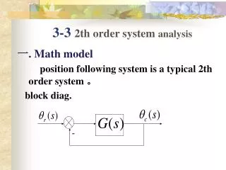
-. 3-3 2th order system analysis. 一 . Math model position following system is a typical 2th order system 。 block diag. Where ξ damped ratio. w n natural oscillation frequency ( also called no damped natural oscillation frequency ). Closed-loop characteristic equ :

E N D
- 3-3 2th order system analysis 一. Math model position following system is a typical 2th order system 。 block diag.
Whereξdamped ratio. wn natural oscillation frequency (also called no damped natural oscillation frequency)
Closed-loop characteristic equ: Its characteristic roots are the poles of closed-loop characteristic equ: 1.when 0< ξ <1,a couple of conjugate complex roots with negative part called under-damped。(fig .a)
2.whenξ=1,2 equal negative roots ,called critically damped。(fig.b) 3. whenξ>1, 2 different negative roots, called over damped。( fig. c) 4. whenξ=0, a couple of conjugate imaginary roots , called non-damped or 0 -damped。(fig.d) following calculate respectively。
二. 2th order system unit step response 1.over-damped。 whenξ>1, 2 different negative roots, closed-loop TF
where: Over damped 2th order system can be seen to have two first order system series with different time constants. When input signal is an unit step
output inverse Laplace transformation:
Starting speed is small, then gradually increases, different from first order system.it is difficult to solve ts, generally use computer to solve it.。 response curve: From the curve,when , when , ,so when It can approximate a first order system. Response is very slowly,little adopted。
2.under-damped When 0< ξ <1,closed-loop characteristic equ. wn natural oscillation frequency (also called no damped natural oscillation frequency) 。
under-damped 2th order system unit step response attenuates to its steady-state value according to exponent rule,attenuating speed depends on -ξwn, attenuating frequency depends on wd。 angle definition
from the curve, ξ ↑,σ%↓;ξ ↓ , σ% ↑ 。When ξ=0,0 damped response is: constant amplitude oscillation curve,, oscillation frequency is wn wn is called no dampedoscillation frequency 。
if ξ ↑↑→ ts ↑ ; if ξ ↓↓→ ts andtp ↓,but σ% ↑ →ts ↑ ↑ 。
1.rise time tr from definition:tr ---first reach steady-state value,set n=1。
When wn is definite,the smallerξ,the smaller tr; When ξ is definite,the bigger wn, the smaller tr. 2.peak time tp ① ②
Differentiate equ.①,set it=0: replace
Tp--first reach peak value,set n=1。 so When wn is definite,the smallerξ,the smaller tp; When ξ is definite,the bigger wn, the smaller tp. 3.over-shootσ%
ξ↑,σ% ↓ ,in general,takeξin 0.4-0.8, σ% in 25%-2.5%。 4.settling time ts from definition: difficult to solve ts,but get the curve between wnts and ξ:
ts not continuous diag. Small ξ change can produce ts change violently.
whenξ=0.68(5% error band)orξ=0.76(2% error band ),ts is the shortest,the system is often designed under damped 。 un-continuous curve is because the small ξ variant can cause ts variant。 when approximately calculate,usually use embracing curve to calculate ts。
take both sides logarithms, get That is: while design system, the ξ is usually selected by request, but settling time by wn.
5.oscillation No.N definition:in ts,half of the No.response curve cross to steady state value. Td:damped oscillation period。
Exam.1:given a unit feedback system.its open-loop TF assume input r(t)=1(t) ,when KA=200,solve transient response performance。When KA changes to 1500 or KA =13.5,how does the transient response performance?
from this,the bigger KA, the smaller ξ, the bigger wn, the smaller tp, the bigger б%,whereas ts seldom changes。 System works with over-damped, tp, б% ,N do not exist, but ts.can be approximately calculated by a first order system with a big time constant T,that is: .
Ts is much longer than the two KA above.although response has no over-shoot,response process is slow,the curve as follows:
KA ↑ , tp ↓, tr ↓,improve speed,but б% ↑. For improving transient performance ,the proportion-differential control or speed feedback control can be adopted ,namely introduce a correction.。
Homework: Chapter 3-6,3-7