Download
1 / 18
180 likes | 184 Views
Introduction to Queueing Theory. Components of a queueing system probability density function (pdf) of interarrival times pdf of service times the number of servers the queueing disciplines the amount of buffer. Intro. to Queueing Theory (cont’d). Notation M : exponential density function

E N D
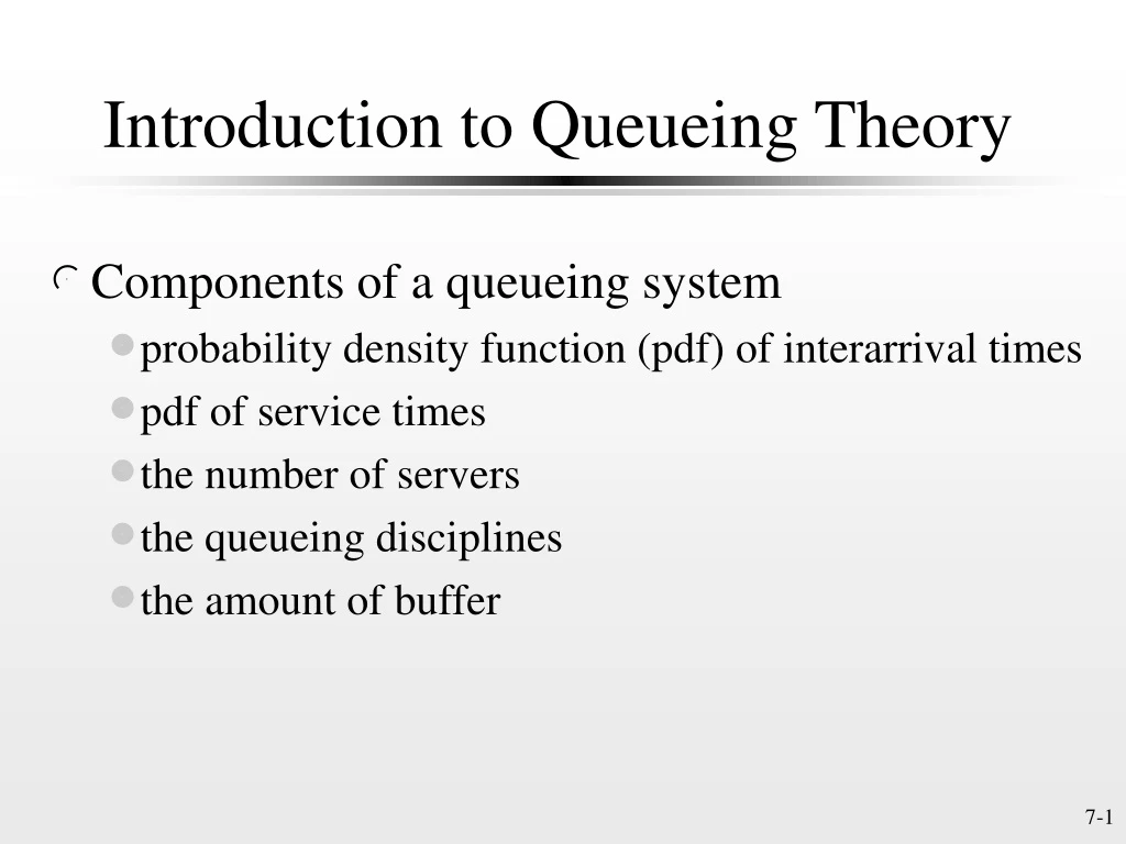
Introduction to Queueing Theory • Components of a queueing system • probability density function (pdf) of interarrival times • pdf of service times • the number of servers • the queueing disciplines • the amount of buffer
Intro. to Queueing Theory (cont’d) • Notation • M: exponential density function • D: deterministic • G: general e.g. M/M/1, M/M/m/m, M/D/1/K, G/G/m • Little’s result: N=T. • M/G/1 queues are fully solvable (P-K formula) • M/M/m/m queueing models can be used to analyze the call blocking probability (Erlang B formula)
Medium Access Sublayer • How to access a multiaccess/random access/ broadcast channel? • Static channel allocation • FDM • low throughput • example: M/M/1 with arrival rate l (frames per sec.) and service rate m (frames per sec.) • Tshared=1/(m-l) for sharing the entire channel • TFDM=1/(m/n-l/n)=n/(m-l)=nTshared for distributing equally the traffic among n identical subchannels (same total cap.)
Medium Access Sublayer (cont’d) • Dynamic channel allocation • station models: N independent Poisson sources (exponential interarrival times) • single channel • errors & retransmissions are caused solely by collisions • continuous time vs. slotted time • with and without carrier sense
Medium Access Sublayer (cont’d) • ALOHA protocols • pure ALOHA • users transmit data whenever they have data to send • collisions can be detected • damaged frames are retransmitted after a random delay • fixed frame size (which leads to the max. throughput) Fig. 4-1, p. 247
Medium Access Sublayer (cont’d) • ALOHA protocols (cont’d) • pure ALOHA (cont’d) • performance analysis S: normalized throughput/offered load (0 S 1) G: S + retransmissions Poisson arrival process with mean rate G (assumed) Pr{k arrivals in a time period of t}=Pk(t)=(Gt)ke-Gt/k! Fig. 4-2, p. 249
Medium Access Sublayer (cont’d) • ALOHA protocols (cont’d) • pure ALOHA (cont’d) Pr{a particular frame is successfully transmitted} = Pr{0 other transmission in its vulnerable period (2)} = e-2G Then, S = Ge-2G. To maximize S dS/dG=e-2G-2G e-2G=(1-2G) e-2G=0. Consequently, G*=0.5and S*=1/2e=18%.
Medium Access Sublayer (cont’d) • ALOHA protocols (cont’d) • slotted ALOHA • the same as pure ALOHA except that data are transmitted at the beginning of a time slot • the vulnerable period is 1 • performance analysis Pr{a particular frame is successfully transmitted} = Pr{0 other transmission in its vulnerable period (1)} = e-G Then, S = Ge-G. To maximize S, dS/dG=e-G-G e-G=(1-G) e-G=0. Consequently, G*=1and S*=1/e=36%.
Medium Access Sublayer (cont’d) • ALOHA protocols (cont’d) • slotted ALOHA (cont’d) • expected number of transmissions of a frame success probability = e-G failure probability = 1 - e-G Assume that the number of transmissions can be characterized by a geometric distribution Pr{k transmissions} = e-G (1- e-G)k-1. mean value = 1/ e-G = eG (delayincreases exponentially with G)
Medium Access Sublayer (cont’d) • Carrier sense multiple access (CSMA) protocols • 1-persistent CSMA (0) Continue. (1) If the station is idle, go to (0). (2) Sense the channel. (3) If the channel is busy, go to (2) [with probability 1]. (4) Send the frame. (5) If there is no collision, go to (1). (6) Delay a random time and go to (2).
Medium Access Sublayer (cont’d) • CSMA protocols (cont’d) • nonpersistent CSMA (0) Continue. (1) If the station is idle, go to (0). (2) Sense the channel. (3) If the channel is busy, delay a random time and go to (2). (4) Send the frame. (5) If there is no collision, go to (1). (6) Delay a random time and go to (2). Achieves better channel throughput but incurs larger delay than 1-persistent CSMA.
Medium Access Sublayer (cont’d) • CSMA protocols (cont’d) • p-persistent CSMA (applied to slotted channels) (0) Continue. (1) If the station is idle, go to (0). (2) Sense the channel. (3) If the channel is busy, wait until the next time slot and go to (2). (4) Generate a uniformly distributed random variable R over interval [0,1]. (5) If p<=R<=1, then wait until the next time slot and sense the channel. If the channel is idle then go to (4). Else send the frame. If there is no collision, go to (1). (6) Delay a random time and go to (2).
Medium Access Sublayer (cont’d) • CSMA protocols (cont’d) • CSMA/CD (CSMA with collision detection) Fig. 4-5, p. 253 • channel seizure time is 2t, where t is the full cable propagation time t0 t0+t- A B t0+2t-
Medium Access Sublayer (cont’d) • Collision-free protocols • bit-map protocol • N contention (reservation) slots, one for each station, before a transmission period • example Fig. 4-6, p. 254 • the length of each contention period is N
Medium Access Sublayer (cont’d) • Collision-free protocols (cont’d) • binary countdown • example Fig. 4-7, p. 256 • the length of each contention period is log2N
Medium Access Sublayer (cont’d) • Limited-contention protocols • objectives • low delay at low load (like contention protocols) • high throughput at high load (like contention-free protocols) • success probability analysis k stations, each transmitting with probability p Let g = Pr{some one transmits successfully} = kp(1-p)k-1. Find g* (optimal) by setting d/dp[kp(1-p)k-1] to 0. Then, p* = 1/k and g* = (1-1/k)k-1. Fig. 4-8, p. 258
Medium Access Sublayer (cont’d) • Limited-contention protocols (cont’d) • basic approaches • divide stations into groups (trying to limit k) • only members of a group are allowed to transmit at a time • the adaptive tree walk protocol • binary trees with depth first search upon collisions • example Fig. 4-9, p. 259
Medium Access Sublayer (cont’d) • Limited-contention protocols (cont’d) • the adaptive tree walk protocol (cont’d) • under low loads, the search should start from the top • under heavy loads, the search should start from the bottom • What is the optimal level to start the search? • Let q be the expected number of ready stations. • Label the levels from the top by 0,1,2,... • For a node at level i, a fraction of 1/2i of the total stations is below it. • An optimal selection of i is to let q/2i=1. • Consequently, i*=log2q. • ways to improve the performance: e.g. node 1: collision & node 2: idle, then skip node 3 (must be collision)