Download
1 / 17
180 likes | 354 Views
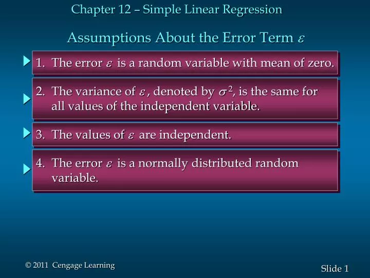
Chapter 12 – Simple Linear Regression. Assumptions About the Error Term e. 1. The error is a random variable with mean of zero. 2. The variance of , denoted by 2 , is the same for all values of the independent variable. 3. The values of are independent.

E N D
Chapter 12 – Simple Linear Regression Assumptions About the Error Term e 1. The error is a random variable with mean of zero. 2. The variance of , denoted by 2, is the same for all values of the independent variable. 3. The values of are independent. 4. The error is a normally distributed random variable.
Testing for Significance To test for a significant regression relationship, we must conduct a hypothesis test to determine whether the value of b1 is zero. Two tests are commonly used: t Test F Test and Both the t test and F test require an estimate of s2, the variance of e in the regression model.
Testing for Significance • An Estimate of 2 • The mean square error (MSE) provides the estimate • of s2, and the notation s2 is also used. s2 = MSE = SSE/(n - 2) where:
Testing for Significance • An Estimate of s • To estimate s we take the square root of s 2. • The resulting s is called the standard error of • the estimate.
Testing for Significance: t Test • Hypotheses • Test Statistic
Testing for Significance: t Test • Rejection Rules p-Value Approach: Reject H0 if p-value <a Critical Value Approach: Reject H0 ift< - t/2or t>t/2 where: tis based on a t distribution with n - 2 degrees of freedom
Testing for Significance: t Test 1. Determine the hypotheses. a = .05 2. Specify the level of significance. 3. Select the test statistic. 4. State the rejection rule. Reject H0 if p-value < .05 or |t| > 3.182 (with 3 degrees of freedom)
Testing for Significance: t Test 5. Compute the value of the test statistic. 6. Determine whether to reject H0. t = 4.541 provides an area of .01 in the upper tail. Hence, the p-value is less than .02. (Also, t = 4.63 > 3.182.) We can reject H0.
Confidence Interval for 1 • We can use a 95% confidence interval for 1 to test • the hypotheses just used in the t test. • H0 is rejected if the hypothesized value of 1 is not • included in the confidence interval for 1.
is the margin of error where is the t value providing an area of a/2 in the upper tail of a t distribution with n - 2 degrees of freedom Confidence Interval for 1 • The form of a confidence interval for 1 is: b1 is the point estimator
= 5 3.182(1.08) = 5 3.44 Confidence Interval for 1 • Rejection Rule Reject H0 if 0 is not included in the confidence interval for 1. • 95% Confidence Interval for 1 or 1.56 to 8.44 • Conclusion 0 is not included in the confidence interval. Reject H0
Testing for Significance: F Test • Hypotheses • Test Statistic F = MSR/MSE MSR = SSR/1
Testing for Significance: F Test • Rejection Rule p-Value Approach: Reject H0 if p-value <a Critical Value Approach: Reject H0 ifF>F where F is the value leaving an area if in the upper tail of theF distribution with 1 degree of freedom in the numerator and n - 2 degrees of freedom in the denominator.
Example: Reed Auto Sales 1. Determine the hypotheses. a = .05 2. Specify the level of significance. 3. Select the test statistic. F = MSR/MSE 4. State the rejection rule. p-Value Method: Reject H0 if p-value < .05 Critical Value Method: Reject H0if F> 10.13 (1 d.f. in numerator and 3 d.f. in denominator)
Example: Reed Auto Sales 5. Compute the value of the test statistic. F = MSR/MSE = 100/4.667 = 21.43 6. Determine whether to reject H0. p-value Method: F = 21.43 lies between the values of 17.44 and 34.12 in the F table, so the p-value is between .025 and .01. Thus, the p-valueis below .05 and we reject H0. Critical Value Method: 21.43 > 10.13 so we reject H0. We have a significant relationship between the number of TV ads aired and the number of cars sold.
Caution about theInterpretation of Significance Tests • Rejecting H0: b1 = 0 and concluding that the • relationship between x and y is significant does not enable us to conclude that a cause-and-effect • relationship is present between x and y.