Download

1 / 63
630 likes | 636 Views
Trees, Binary Trees, and Binary Search Trees. Trees. Linear access time of linked lists is prohibitive Does there exist any simple data structure for which the running time of most operations (search, insert, delete) is O(log N)? Trees Basic concepts Tree traversal Binary tree

E N D
Trees • Linear access time of linked lists is prohibitive • Does there exist any simple data structure for which the running time of most operations (search, insert, delete) is O(log N)? • Trees • Basic concepts • Tree traversal • Binary tree • Binary search tree and its operations
Trees • A tree T is a collection of nodes • T can be empty • (recursive definition) If not empty, a tree T consists of • a (distinguished) node r (the root), • and zero or more nonempty sub-trees T1, T2, ...., Tk
Tree can be viewed as a ‘nested’ lists: • list of lists of lists … • Tree is also a graph …
Some Terminologies • Child and Parent • Every node except the root has one parent • A node can have a zero or more children • Leaves • Leaves are nodes with no children • Sibling • nodes with same parent
More Terminologies • Path • A sequence of edges • Length of a path • number of edges on the path • Depth of a node • length of the unique path from the root to that node • Height of a node • length of the longest path from that node to a leaf • all leaves are at height 0 • The height of a tree = the height of the root = the depth of the deepest leaf • Ancestor and descendant • If there is a path from n1 to n2 • n1 is an ancestor of n2, n2 is a descendant of n1 • Proper ancestor and proper descendant
Tree Operations • Traversal, the most important • we will not implement a general ‘tree’, so wont discuss • Search • Insertion • Deletion
Tree Traversal • Used to print out the data in a tree in a certain order • Pre-order traversal • Print the data at the root • Recursively print out all data in the leftmost subtree • … • Recursively print out all data in the rightmost subtree
A drawing of tree with two pointers … Struct TreeNode { double element; // the data TreeNode* child; // FIRST child : go to the next generation TreeNode* next; // next SIBLING : go to the same generation }
preorder(tree) if empty(tree) stop else print(element(tree)) preorder(child(tree)) preorder(next(tree))
Example: Unix Directory Traversal PreOrder PostOrder
Binary Trees • A tree in which no node can have more than two children • The depth of an “average” binary tree is considerably smaller than N, even though in the worst case, the depth can be as large as N – 1. Generic binary tree Worst-casebinary tree
Binary Tree ADT • Implementation • at most two children, we can keep direct pointers to them • a linked list is physically a pointer, so is a tree! • Possible operations on the Binary Tree ADT • Parent, left_child, right_child, sibling, root, etc • Tree operations: • Search, insertion and deletion • Make a Binary Tree ADT later …
A drawing of linked list with one pointer … A drawing of binary tree with two pointers … Struct BinaryNode { double element; // the data BinaryNode* left; // left child BinaryNode* right; // right child }
Example: Expression Trees • Leaves are operands (constants or variables) • The internal nodes contain operators • Will not be a binary tree if some operators are not binary
Preorder, Postorder and Inorder • Preorder traversal • node, left, right • prefix expression • ++a*bc*+*defg
Postorder traversal left, right, node postfix expression abc*+de*f+g*+ Inorder traversal left, node, right infix expression a+b*c+d*e+f*g Preorder, Postorder and Inorder
Recall the binary search algorithm 4 7 10 15 19 20 42 54 87 90
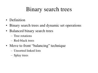
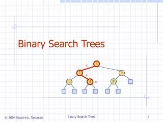
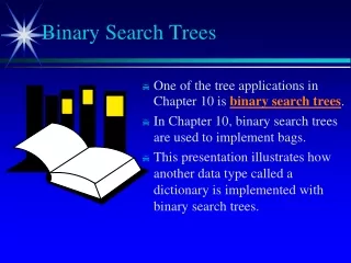
Binary Search Trees (BST) • A data structure for efficient searching, inser-tion and deletion • Binary search tree property • For every node X • All the keys in its left subtree are smaller than the key value in X • All the keys in its right subtree are larger than the key value in X
Binary Search Trees A binary search tree Not a binary search tree
Binary Search Trees The same set of keys may have different BSTs • Average depth of a node is O(log N) • Maximum depth of a node is O(N)
Searching BST • If we are searching for 15, then we are done. • If we are searching for a key < 15, then we should search in the left subtree. • If we are searching for a key > 15, then we should search in the right subtree.
Searching (Find) • Find X: return a pointer to the node that has key X, or NULL if there is no such node • Time complexity: O(height of the tree) find(const double x, BinaryNode* t) const
Inorder Traversal of BST • Inorder traversal of BST prints out all the keys in sorted order Inorder: 2, 3, 4, 6, 7, 9, 13, 15, 17, 18, 20
findMin/ findMax • Goal: return the node containing the smallest (largest) key in the tree • Algorithm: Start at the root and go left (right) as long as there is a left (right) child. The stopping point is the smallest (largest) element • Time complexity = O(height of the tree) BinaryNode* findMin(BinaryNode* t) const
Insertion • Proceed down the tree as you would with a find • If X is found, do nothing (or update something) • Otherwise, insert X at the last spot on the path traversed • Time complexity = O(height of the tree)
void insert(double x, BinaryNode*& t) { if (t==NULL) t = new BinaryNode(x,NULL,NULL); else if (x<t->element) insert(x,t->left); else if (t->element<x) insert(x,t->right); else ; // do nothing }
Insertion Example Construct a BST successively from a sequence of data: 35,60,2,80,40,85,32,33,31,5,30
Deletion • When we delete a node, we need to consider how we take care of the children of the deleted node. • This has to be done such that the property of the search tree is maintained.
Deletion under Different Cases • Case 1: the node is a leaf • Delete it immediately • Case 2: the node has one child • Adjust a pointer from the parent to bypass that node
Deletion Case 3 • Case 3: the node has 2 children • Replace the key of that node with the minimum element at the right subtree • (or replace the key by the maximum at the left subtree!) • Delete that minimum element • Has either no child or only right child because if it has a left child, that left child would be smaller and would have been chosen. So invoke case 1 or 2. • Time complexity = O(height of the tree)
void remove(double x, BinaryNode*& t) { if (t==NULL) return; if (x<t->element) remove(x,t->left); else if (t->element < x) remove (x, t->right); else if (t->left != NULL && t->right != NULL) // two children { t->element = finMin(t->right) ->element; remove(t->element,t->right); } else { Binarynode* oldNode = t; t = (t->left != NULL) ? t->left : t->right; delete oldNode; } }
Deletion Example 30 30 5 5 40 60 2 80 2 80 35 35 32 32 85 85 60 33 33 31 31 (b) (a) Removing 40 from (a) results in (b) using the smallest element in the right subtree (i.e. the successor)
30 30 5 5 35 40 2 80 32 2 80 35 32 85 60 31 33 60 85 33 31 (c) (a) Removing 40 from (a) results in (c) using the largest element in the left subtree (i.e., the predecessor) 39
30 5 5 2 35 35 80 2 80 32 32 31 31 33 33 60 60 85 85 (d) (c) Removing 30 from (c), we may replace the element with either 5 (predecessor) or 31 (successor). If we choose 5, then (d) results. 40
Example: Successor The successor of a node x is defined as: The node y, whose key(y) is the successor of key(x) in sorted order sorted order of this tree. (2,3,4,6,7,9,13,15,17,18,20) Some examples: Which node is the successor of 2? Which node is the successor of 9? Which node is the successor of 13? Which node is the successor of 20? Null Search trees 42
Scenario I: Node x Has a Right Subtree By definition of BST, all items greater than x are in this right sub-tree. Successor is the minimum( right( x ) ) maybe null Search trees 43
Scenario II: Node x Has No Right Subtree and x is the Left Child of Parent (x) Successor is parent( x ) Why? The successor is the node whose key would appear in the next sorted order. Think about traversal in-order. Who wouldbe the successor of x? The parent of x! Search trees 44
Scenario III: Node x Has No Right Subtree and Is Not a Left-Child of an Immediate Parent Keep moving up the tree until you find a parent which branches from the left(). Successor of x y Stated in Pseudo code. x Search trees 45
Three Scenarios to Determine Successor Successor(x) x has right descendants => minimum( right(x) ) x has no right descendants Scenario I x is the left child of some node => parent(x) x is the right child of some node Scenario II Scenario III Search trees 46
Successor Pseudo-Codes Verify this code with this tree. Find successor of 3 4 9 13 13 15 18 20 Note that parent( root ) = NULL Scenario I Scenario II Scenario III Search trees 47
Problem If we use a “doubly linked” tree, finding parent is easy. But usually, we implement the tree using only pointers to the left and right node. So, finding the parent is tricky. For this implementation we need to store the ‘path’ Stack! class Node { int data; Node * left; Node * right; Node * parent; }; class Node { int data; Node * left; Node * right; }; 48
Use a Stack to Find Successor PART I Initialize an empty Stack s. Start at the root node, and traverse the tree until we find the node x. Push all visited nodes onto the stack. PART II Once node x is found, find successor using 3 scenarios mentioned before. Parent nodes are found by popping the stack! 49
Example Successor(root, 13) Part I Traverse tree from root to find 13 order -> 15, 6, 7, 13 7 6 15 Stack s 50