Download
1 / 52
1.97k likes | 4.17k Views
INVENTORY MODELS. Inventory. Inventory is any kind of resource which has economic value and is maintained to fulfill the present and future requirements. Inventory can be physical, human or financial.

E N D
Inventory • Inventory is any kind of resource which has economic value and is maintained to fulfill the present and future requirements. • Inventory can be physical, human or financial. • Inventory is necessary evil – too little can cause disruptions and too much can cause bankruptcy. • Maintaining right inventory is strategic for the organization. INVENTORY MODELS
Inventory Control • What items need to be stocked • Based on criticality, cost, supplier, strategy etc. • How much to order of each material when orders are placed with either outside suppliers or production departments within organizations? • Depends on demand pattern, lead time, price, inventory costs. • When to place the orders • Depends on the review mechanism • Periodic review, Fixed order quantity INVENTORY MODELS
Types of Inventory • Lot size or Cycle Inventory – Inventory kept to meet the average demand during replenishment period. • Pipeline or Transit Inventory – Inventory kept to meet the shortfall due to inventory in transit, (work in process) • Safety Inventory – To meet the uncertainties of demand. • Seasonal Inventory – to meet seasonal demands INVENTORY MODELS
Independent Demand Dependent Demand A C(2) B(4) D(2) E(1) D(3) F(2) Independent demand is uncertain. Dependent demand is certain. Types of Demand INVENTORY MODELS
Reasons for carrying inventory • Improve customer service • Reduce certain costs such as • ordering costs • stock out costs • acquisition costs • quantity costs • start-up quality costs • Contribute to the efficient and effective operation of the production system by decoupling the subsets. INVENTORY MODELS
Reasons for avoiding inventory • Higher costs • Interest or opportunity costs • Holding (or carrying) costs – storage, handling, taxes, insurance, shrinkage • Ordering (or setup) costs • Risk of deterioration or obsolescence • Hides production problems • Yield / scrap variations • Unscheduled downtime INVENTORY MODELS
Counterviews on Inventory • Pressure for lower inventory • Inventory investment • Inventory holding cost • Pressure for higher inventory • Customer service • Other costs related to inventory INVENTORY MODELS
Effective Inventory Management • A system to keep track of inventory • A reliable forecast of demand • Knowledge of lead times • Reasonable estimates of • Holding costs • Ordering costs • Shortage costs • A classification system INVENTORY MODELS
Features of Inventory System • Relevant inventory costs. • Demand Pattern • Replenishment lead time • Length of planning period • Constraint on the inventory system. INVENTORY MODELS
Inventory System • Purchase cost • Ordering cost • Holding cost • Shortage cost System Performance Replenishment plan Inventory system Demand Pattern • Constant • Instantaneous • Uniform • Deterministic • Probabilistic Operating decision rules Operating Constraints Buffer Stock Safety Stock Reserve stock Customer Service level When to order How much to order INVENTORY MODELS
Inventory Decision Rules INVENTORY MODELS
Relevant Inventory Costs • Purchase Costs Quantity discounts. • Carrying or holding costs – Storage, deterioration, loss, pilferage, demurrage, and others. • Carrying cost = Cost of carrying one unit for a given time x Average no of units carried in that period • Ordering or Set up costs • Shortage cost or stock out – Loss of goodwill or loss of customers, Back ordering. • Total Inventory Costs = Purchase Costs + Carrying Costs + Ordering Costs + Shortage Costs • Total Variable Inventory costs = Ordering cost + Carrying costs + Shortage Costs INVENTORY MODELS
Demand Pattern • Size of demand is referred to the no of items required in each period (cycle). • Size of demand may be deterministic or probabilistic. • Deterministic demand can be fixed or varying with time. • Demand can be satisfied simultaneously or can be replenished over period of time. INVENTORY MODELS
Order Cycle • Order cycle is the time period between two successive orders. • Continuous review – In this case an order of fixed quantity is placed every time the inventory reaches a pre-defined level. Referred as Two-bin system, Fixed order size system or Q-system • Periodic Review – In this case the orders are placed at regular interval but the order quantity is varying with variations in demand. Referred as Fixed order interval system or P-system. INVENTORY MODELS
Inventory Model Building • Objective is to determine the order quantity that minimizes cost. • Collect data regarding the pattern of demand, replenishment policy, planning period, costs related to inventory and any constraints. • Build a mathematical model using any of the analytical tools applicable. • Derive the optimal inventory policy. INVENTORY MODELS
Economic Order Quantity (EOQ) • EOQ concept developed by Ford Harris in 1913. • Concept is to balance the cost of holding excess costs against that of ordering costs. • EOQ models have evolved over the period for overcoming the simplistic assumptions. • EOQ is the size of the order that yields the optimum total incremental inventory cost during the given period of time under the assumption that demand rate is constant. INVENTORY MODELS
Inventory models Inventory control models Models without price quantity discounts Models with price quantity discount Probabilistic Demand Models Deterministic demand models Static demand models Dynamic demand models Variable demand with constant lead time model Fixed order qty with variable LT Fixed Interval ordering model with variable lead time Models with no shortage Models with shortage Resource constraints models INVENTORY MODELS
Inventory Models Models without Shortage Models with Shortage • Variable order cycle time, supply is instantaneous • Constant order cycle time and supply is uniform • Demand rate is uniform but supply is non-instantaneous • Demand rate constant in all cycles, supply is instantaneous • Different rates of demand in different cycles but total demand is known over the entire planning period • Demand rate is constant but supply is non-instantaneous INVENTORY MODELS
Basic Notations • C = purchase or manufacturing cost per unit (Rs/unit) • Co= ordering cost or set up cost per order (Rs/order) • Ch= cost of carrying one unit of item in inventory for a given length of time (Rs/unit time) • r=cost of carrying one rupee’s worth of inventory per time period (usually expressed in terms of percent of rupee value of inventory) (percent/time) • Cs= shortage cost per unit per time (Rs/unit-time) • D= annual requirement • Q= order quantity no of units ordered per order. • ROL= reorder level • LT= replenishment lead time • n= no of orders per unit time (orders/time) • t= reorder cycle time (time interval between successive orders) • tp=production period (time period) • rp= production rate • TC= total inventory cost, TVC = Total variable inventory cost INVENTORY MODELS
Model with constant demand • Objective is to find EQO Q*, which minimizes cost • Assumptions are • Only one product is involved • Demand requirements known and constant rate per time period • Demand is even throughout the year • Lead time does not vary • Each order is received in a single delivery • There are no quantity discounts • Shortages are not allowed. • Each item is independent and no saving possible by substitution. INVENTORY MODELS
BASIC EOQ MODEL Usage Rate Order Placed Inventory Level Maximum Inventory Level Q Average Inventory = Q/2 0 Time t Lead Time INVENTORY MODELS
Cost Curves Total cost = HC + OC Annual cost (dollars) Holding cost (HC) Ordering cost (OC) Lot Size (Q) INVENTORY MODELS
Derivation of EOQ INVENTORY MODELS
EXAMPLE 1 • A computer company has annual demand of 10,000. They want to determine EOQ for circuit boards which have an annual holding cost (H) of Rs 6 per unit, and an ordering cost (S) of Rs 75. They want to calculate TC and the reorder point (R) if the purchasing lead time is 5 days. INVENTORY MODELS
Model with different Demand Rates • The demand is constant with different rates in different cycles. • Let q be the constant demand in different time periods t1, t2…tn. • t1+t2+…tn= T, the total planning period. • D= D1+D2+…Dn, total demand. • Carrying cost = 1/2qt1Ch+1/2qt2Ch+…+1/2qtnCh =1/2qChT • Set up cost = D/q x Co INVENTORY MODELS
Inventory Level with different Demand Rates Maximum Inventory Level Q 0 Time t2 t1 INVENTORY MODELS
EOQ Model with non-instantaneous supply • Also termed as Economic Production Quantity • Production done in batches or lots • Capacity to produce a part exceeds the part’s usage or demand rate • Supplies are received in several shipments. • Assumptions of EPQ are similar to EOQ except orders are received incrementally during production • Supply is constant and constant until Q units are supplied in stock. • The rate of receipt p of replenishment of stocks is greater than rate of usage d. • Production begins immediately after set up. INVENTORY MODELS
Graphical Representation of EOQ d tp Reorder level Production cycle time t INVENTORY MODELS
Derivation of EPQ INVENTORY MODELS
Example 2 • A contractor has to supply 10000 bearings per day to an automobile manufacturer. He finds that when he starts production run, he can produce 25000 bearings per day. The cost of holding a bearing in stock per year is Rs. 2 and the set up costs for a production run is Rs. 1800. How frequently should production run be made? INVENTORY MODELS
EOQ With Price Discounts • Under quantity discounts, a supplier offers a lower unit price if larger quantities are ordered at one time • This is presented as a price or discount schedule, i.e., a certain unit price over a certain order quantity range • This means this model differs from earlier Model because the acquisition cost may vary with the quantity ordered, i.e., it is not necessarily constant. • Quantity discounts may be for all units or for incremental quantity. • Assumptions are demand is constant, shortage are not allowed, and replenishment is instantaneous. INVENTORY MODELS
EOQ With Price Discounts INVENTORY MODELS
EOQ with Price Discounts • The first model is where we have price discounts available for all units between a certain quantity. • The above model cannot be solved by simple calculus. • We have to estimate the total cost for each price break and do it iteratively. • Total Cost Tci (Q)=Direct Cost up to unit i + Total variable cost. • Tci=DCi +sqrt (2DCo(rCi)) INVENTORY MODELS
Model with One Price break • Suppose the supplier offers a price discount at quantity b1 • This means that up to qty b1 the price is say C1 and beyond the qty b1 the price is C2 (<C1). • The method of calculating EOQ is as follows: • Calculate the EOQ (Q2*) with lowest price (C2). If this lies in the prescribed range, b1<Q2*, then Q2* is the EOQ. • If Q2* is not equal to or more than b1, then calculate EOQ (Q1*) with price C1. INVENTORY MODELS
Calculating Total Cost with PD • If Q2* lies in the range b1<Q2* then TC* is • TC*= (TC2*)= DC2 + D/b1 Co + b1/2 (C2 x r) • If Q2* is not equal to or more than b1 then TC* is given by • TC(Q1*) =DC1 + D/Q1* Co + Q1*/2 (C1 x r) • TC (b1) = DC2 + D/b1 Co + b1/2 (C2 x r) • Compare TC(b1) with TC(Q1*). • If TC (b1) > TC (Q1*) then EOQ is Q1*, else it is b1. INVENTORY MODELS
Example 3 • The annual demand of the product is 10000 units. Each unit costs Rs 100 if orders placed in quantities below 200 units. For orders above 200 units the price is Rs. 95. The annual inventory holding cost is 10 % of the value of the item. Ordering cost is Rs 5 per order. Find the economic lot size. INVENTORY MODELS
Determinants of the Reorder Point • The rate of demand • The lead time • Demand and/or lead time variability • Stockout risk (safety stock) INVENTORY MODELS
Dynamic Demand Inventory Models • Reorder Level with Constant demand • Till now we have calculated the EOQ, how much to order. • Now we need to know when to reorder. • In a continuous review system when the inv level reaches a particular level called ROL, a new order is placed. • The effective level of inventory a particular point of time is stock in hand plus stock on order minus the outstanding orders INVENTORY MODELS
Reorder Level with Constant Demand • Reorder Level will be equal to lead time demand. • Lead time demand = demand rate x Lead time • The above rule works when LT is less than stock cycle. • If stock cycle is greater than lead time then in every consumption cycle we will have one order outstanding. • LTD=Stock in hand + Stock on order INVENTORY MODELS
Service Level • Service Level is applicable when demand is uncertain and shortage costs are difficult to estimate. • Service Level is the probability of meeting the demand during an inventory cycle. • It is also the probability that the demand during lead time will be less than ROL. • It takes values between 0 to 1. • Role of service levels is used to decide the additional stocks required to meet the target. INVENTORY MODELS
Additional Stocks • When demand is uncertain and lead time is not certain then we maintain additional stocks. • Reserve Stock is taken to meet the variations in demand. • Safety Stock is used to meet the variations of lead time. • The above types of stocks are determined using • Probability of known and unknown shortages. • Desired customer service level • Probability of delay in lead time • Maximum delay in lead time INVENTORY MODELS
Additional Stocks • Buffer Stock is the additional stock kept based on the average demand rate for the total period. • Buffer Stock = Average Demand x Average Lead Time. • When no stock outs are preferred then buffer stock is given by • BS = (max demand during LT – ave demand during LT) • Thus ROL using BS is given by • ROL = dav x LT +BS, where dav is average demand during LT INVENTORY MODELS
Example 4 • Annual demand is 12000 units. Ordering cost Rs 60 per order. Carrying cost is 10%. Unit cost is Rs. 10 and LT is 10 days. There are 300 working days in the year. Determine EOQ and no of orders per year. In the recent months the demand has reached 70 units per day. For a reordering system based on inv level what should be the buffer stock? What should be the reorder level at this buffer stock? What would be the carrying costs? INVENTORY MODELS
When to Reorder with EOQ Ordering • Reorder Point - When the quantity on hand of an item drops to this amount, the item is reordered • Safety Stock - Stock that is held in excess of expected demand due to variable demand rate and/or lead time. • Service Level - Probability that demand will not exceed supply during lead time. INVENTORY MODELS
Inventory Control Approaches • Fixed Order Quantity Approach • A record of inventory is maintained regularly. • As soon as the effective inv level drops to a specified level called “reorder level”, a replenishment order of quantity Q* is placed. • There is a risk of stock out if the lead time varies. • The probability of the LT variation is controlled by raising or lowering the ROL. • The objective is to determine the ROL using the probability of LT variation • ROL = Ave demand during LT + Reserve stock + Safety stock. • This system is also called as Perpetual Inventory control system or Continuous Review System INVENTORY MODELS
Fixed Order Quantity Approach • Determination of reserve stock and reorder level • Reserve stock with known stock out costs • Determine the discrete probability distribution function for demand during the reorder LT. • Calculate the optimal reorder level in terms of least expected inventory costs which is carrying cost plus shortage costs. • Then Reserve stock is given • RS = Reorder Level – Average Demand during LT (DDLT) • Ave DDLT = ∑ dLT P(dLT), where dLT is demand during lead time and P(dLT) is probability during reorder lead time INVENTORY MODELS
Fixed Order Quantity Approach • Reorder Level with uncertain demand • To determine reorder level it is necessary to establish tradeoff between cost of carrying reserve stock and the cost of stockouts. • Expected shortage cost from nth item of reserve stock is = Cs x P{dLT > (μLT +n)} where • Cs = cost of shortage, dLT = actual demand during LT, μLT = expected demand during LT and n= nth unit of reservve stock. • The units to reserve stock are added until the expected increase in inventory holding cost exceeds the expected reduction in stock out costs. INVENTORY MODELS
Safety Stock INVENTORY MODELS
Quantity Maximum probable demand during lead time Expected demand during lead time ROP Safety stock Time LT Safety Stock INVENTORY MODELS