Download
1 / 69
690 likes | 846 Views
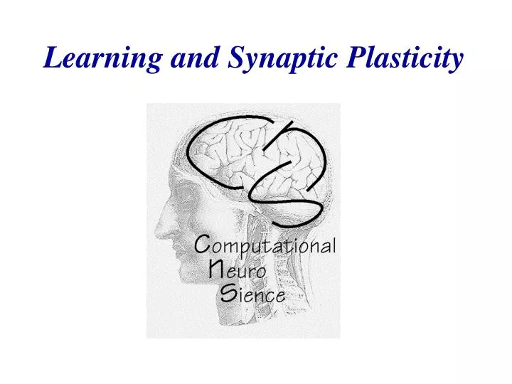
Learning and Synaptic P lasticity. Levels of Information Processing in the Nervous System. 1m. CNS. 10cm. Sub-Systems. 1cm. Areas / „Maps“ . 1mm. Local Networks. 100 m m. Neurons. 1 m m. Synapses. 0.01 m m. Molecules. Structure of a Neuron:. At the dendrite the incoming

E N D
Levels of Information Processing in the Nervous System 1m CNS 10cm Sub-Systems 1cm Areas / „Maps“ 1mm Local Networks 100mm Neurons 1mm Synapses 0.01mm Molecules
Structure of a Neuron: At the dendrite the incoming signals arrive (incoming currents) At the soma current are finally integrated. At the axon hillock action potential are generated if the potential crosses the membrane threshold The axon transmits (transports) the action potential to distant sites CNS Systems At the synapses are the outgoing signals transmitted onto the dendrites of the target neurons Areas Local Nets Neurons Synapses Molekules
Schematic Diagram of a Synapse: Receptor ≈ Channel Transmitter Axon Vesicle Dendrite Transmitter, Receptors, Vesicles, Channels, etc. synaptic weight:
Different Types/Classes of Learning • Unsupervised Learning (non-evaluative feedback) • Trial and Error Learning. • No Error Signal. • No influence from a Teacher, Correlation evaluation only. • Reinforcement Learning (evaluative feedback) • (Classic. & Instrumental) Conditioning, Reward-based Lng. • “Good-Bad” Error Signals. • Teacher defines what is good and what is bad. • Supervised Learning (evaluative error-signal feedback) • Teaching, Coaching, Imitation Learning, Lng. from examples and more. • Rigorous Error Signals. • Direct influence from a teacher/teaching signal.
dwi = m ui v m << 1 Basic Hebb-Rule: dt A reinforcement learning rule (TD-learning): One input, one output, one reward. A supervised learning rule (Delta Rule): No input, No output, one Error Function Derivative, where the error function compares input- with output- examples. An unsupervised learning rule: For Learning: One input, one output.
Learning Speed Autonomy Correlation based learning: No teacher Reinforcement learning , indirect influence Reinforcement learning, direct influence Supervised Learning, Teacher Programming The influence of the type of learning on speed and autonomy of the learner
Hebbian learning When an axon of cell A excites cell B and repeatedly or persistently takes part in firing it, some growth processes or metabolic change takes place in one or both cells so that A‘s efficiency ... is increased. Donald Hebb (1949) A B A t B
Overview over different methods You are here !
…correlates inputs with outputs by the… dw1 = m v u1m << 1 …Basic Hebb-Rule: dt Hebbian Learning w1 u1 v Vector Notation Cell Activity: v = w.u This is a dot product, where w is a weight vector and u the input vector. Strictly we need to assume that weight changes are slow, otherwise this turns into a differential eq.
dw1 Single Input = m v u1m << 1 dt dw = m v um << 1 Many Inputs dt As v is a single output, it is scalar. dw Averaging Inputs = m <v u> m << 1 dt We can just average over all input patterns and approximate the weight change by this. Remember, this assumes that weight changes are slow. If we replace v with w.u we can write: dw = m Q.wwhere Q = <uu> is the input correlation matrix dt Note: Hebb yields an instable (always growing) weight vector!
Synaptic plasticity evoked artificially Examples of Long term potentiation (LTP) and long term depression (LTD). LTP First demonstrated by Bliss and Lomo in 1973. Since then induced in many different ways, usually in slice. LTD, robustly shown by Dudek and Bear in 1992, in Hippocampal slice.
LTP and Learninge.g. Morris Water Maze Blocked LTP Control Learn the position of the platform platform 2 1 rat 4 3 Time per quadrant (sec) 3 1 2 4 3 1 2 4 Before learning After learning Morris et al., 1986
Schematic Diagram of a Synapse: Receptor ≈ Channel Transmitter Axon Vesicle Dendrite Transmitter, Receptors, Vesicles, Channels, etc. synaptic weight:
Synaptic Plasticity: Dudek and Bear, 1993 LTP (Long-Term Potentiation) LTD (Long-Term Depression) 10 Hz LTP LTD
Pre Post tPre tPost Pre Post tPre tPost Conventional LTP = Hebbian Learning Synaptic change % Symmetrical Weight-change curve The temporal order of input and output does not play any role
Markram et. al. 1997 Spike timing dependent plasticity - STDP +10 ms -10 ms
Synaptic Plasticity: STDP LTP Neuron A Neuron B Synapse u v ω LTD Makram et al., 1997 Bi and Poo, 2001
Pre Post tPre tPost Pre Post tPre Pre precedes Post: Long-term Potentiation tPost Pre follows Post: Long-term Depression Spike Timing Dependent Plasticity: Temporal Hebbian Learning Synaptic change % Acausal Causal (possibly) Time difference T [ms]
Back to the Math. We had: dw1 Single Input = m v u1m << 1 dt dw = m v um << 1 Many Inputs dt As v is a single output, it is scalar. dw Averaging Inputs = m <v u> m << 1 dt We can just average over all input patterns and approximate the weight change by this. Remember, this assumes that weight changes are slow. If we replace v with w.u we can write: dw = m Q.wwhere Q = <uu> is the input correlation matrix dt Note: Hebb yields an instable (always growing) weight vector!
Covariance Rule(s) Normally firing rates are only positive and plain Hebb would yield only LTP. Hence we introduce a threshold to also get LTD dw = m (v - Q) um << 1 Output threshold dt v <Q: homosynaptic depression dw = m v (u - Q)m << 1 Input vector threshold dt u <Q: heterosynaptic depression Many times one sets the threshold as the average activity of some reference time period (training period) Q = <v> or Q = <u> together with v = w .u we get: dw = mC .w, where C is the covariance matrix of the input dt C = <(u-<u>)(u-<u>)> = <uu> - <u2> = <(u-<u>)u>
The covariance rule can produce LTD without (!) post-synaptic input. This is biologically unrealistic and the BCM rule (Bienenstock, Cooper, Munro) takes care of this. BCM- Rule dw = m vu (v - Q) m << 1 dt Experiment BCM-Rule dw v post ≠ pre u Dudek and Bear, 1992
The covariance rule can produce LTD without (!) post-synaptic input. This is biologically unrealistic and the BCM rule (Bienenstock, Cooper, Munro) takes care of this. BCM- Rule dw = m vu (v - Q) m << 1 dt As such this rule is again unstable, but BCM introduces a sliding threshold dQ = n (v2 - Q) n < 1 dt Note the rate of threshold change n should be faster than then weight changes (m), but slower than the presentation of the individual input patterns. This way the weight growth will be over-dampened relative to the (weight – induced) activity increase.
less input leads to shift of threshold to enable more LTP Kirkwood et al., 1996 open: control condition filled: light-deprived BCM is just one type of (implicit) weight normalization.
Evidence for weight normalization: Reduced weight increase as soon as weights are already big (Bi and Poo, 1998, J. Neurosci.) Problem: Hebbian Learning can lead to unlimited weight growth. Solution: Weight normalizationa) subtractive (subtract the mean change of all weights from each individual weight). b) multiplicative (mult. each weight by a gradually decreasing factor).
ORI OD Examples of Applications • Kohonen (1984). Speech recognition - a map of phonemes in the Finish language • Goodhill (1993) proposed a model for the development of retinotopy and ocular dominance, based on Kohonen Maps (SOM) • Angeliol et al (1988) – travelling salesman problem (an optimization problem) • Kohonen (1990) – learning vector quantization (pattern classification problem) • Ritter & Kohonen (1989) – semantic maps Program
Differential Hebbian Learningof Sequences Learning to act in response to sequences of sensor events
Overview over different methods You are here !
History of the Concept of Temporally Asymmetrical Learning: Classical Conditioning I. Pawlow
History of the Concept of Temporally Asymmetrical Learning: Classical Conditioning Correlating two stimuli which are shifted with respect to each other in time. Pavlov’s Dog: “Bell comes earlier than Food” This requires to remember the stimuli in the system. Eligibility Trace: A synapse remains “eligible” for modification for some time after it was active (Hull 1938, then a still abstract concept). I. Pawlow
Conditioned Stimulus (Bell) X Stimulus Trace E + w1 Dw1 S S Response w0 = 1 Unconditioned Stimulus (Food) Classical Conditioning: Eligibility Traces The first stimulus needs to be “remembered” in the system
History of the Concept of Temporally Asymmetrical Learning: Classical Conditioning Eligibility Traces Note: There are vastly different time-scales for (Pavlov’s) behavioural experiments: Typically up to 4 seconds as compared to STDP at neurons: Typically 40-60 milliseconds (max.) I. Pawlow
k k k Defining the Trace In general there are many ways to do this, but usually one chooses a trace that looks biologically realistic and allows for some analytical calculations, too. EPSP-like functions: a-function: Shows an oscillation. Dampened Sine wave: Double exp.: This one is most easy to handle analytically and, thus, often used.
Mathematical formulation of learning rules is similar but time-scales are much different. Overview over different methods
V’(t) x Differential Hebb Learning Rule Simpler Notation x = Input u = Traced Input Xi w V ui Early: “Bell” S X0 u0 Late: “Food”
u w Convolution used to define the traced input, Correlation used to calculate weight growth.
Filtered Input Derivative of the Output T Differential Hebbian Learning Output Produces asymmetric weight change curve (if the filters h produce unimodal „humps“)
Pre Post tPre tPost Pre Post tPre tPost Conventional LTP Synaptic change % Symmetrical Weight-change curve The temporal order of input and output does not play any role
Filtered Input Derivative of the Output T Differential Hebbian Learning Output Produces asymmetric weight change curve (if the filters h produce unimodal „humps“)
Pre Post tPre tPost Pre Post tPre Pre precedes Post: Long-term Potentiation tPost Pre follows Post: Long-term Depression Spike-timing-dependent plasticity(STDP): Some vague shape similarity Synaptic change % T=tPost - tPre ms Weight-change curve(Bi&Poo, 2001)
You are here ! Overview over different methods
Presynaptic Signal (Glu) Postsynaptic: Source of Depolarization The biophysical equivalent of Hebb’s postulate Plastic Synapse NMDA/AMPA Pre-Post Correlation, but why is this needed?
Plasticity is mainly mediated by so called N-methyl-D-Aspartate (NMDA) channels. These channels respond to Glutamate as their transmitter and they are voltage depended: