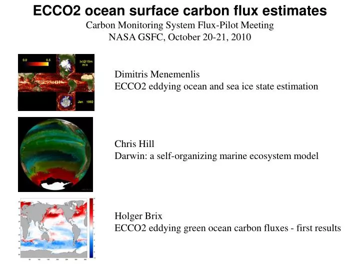
ECCO2 ocean surface carbon flux estimates Carbon Monitoring System Flux-Pilot Meeting

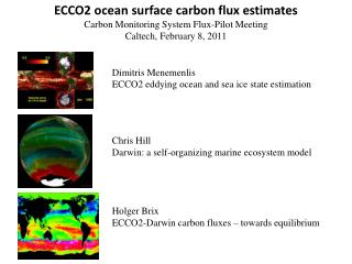
1. ECCO2 ocean surface carbon flux estimates Carbon Monitoring System Flux-Pilot Meeting NASA GSFC, October 20-21, 2010 Dimitris Menemenlis ECCO2 eddying ocean and sea ice state estimation Chris Hill Darwin: a self-organizing marine ecosystem model Holger Brix ECCO2 eddying green ocean carbon fluxes - first results

2. ECCO2: High-Resolution Global-Ocean and Sea-Ice Data Synthesis Objective:synthesis of global-ocean and sea-ice data that covers the full ocean depth and that permits eddies. Motivation: improved estimates and models of ocean carbon cycle, understand recent evolution of polar oceans, monitor time-evolving term balances within and between different components of Earth system, etc. • Forward model: • MITgcm • cubed-sphere • configuration • 18-km • horizontal grid • 50 vertical • levels • modified Leith • viscosity • KPP vertical • mixing • dynamic- • thermodynamic • sea ice Velocity (m/s) At 15 m depth

3. 1992-present eddying global-ocean and sea-ice solution obtained using a Green’s function approach • Data constraints: • sea level anomaly • time-mean sea level • - sea surface temperature • temperature/salinity profiles • sea ice concentration • sea ice motion • sea ice thickness • ~80 control parameters: • initial temperature and salinity conditions • - atmospheric surface boundary conditions • background vertical diffusivity • - critical Richardson numbers for Large et al. (1994) KPP scheme • - air-ocean, ice-ocean, air-ice drag coefficients • ice/ocean/snow albedo coefficients • - bottom drag and vertical viscosity

4. Eddying, global-ocean, and sea ice solution obtained using the adjoint method to adjust ~109 control parameters Cost functions reduction during first 22 forward-adjoint iterations • Baseline solution derived from optimized Green’s function solution and OCCA (Forget 2010) climatology • Optimization period is beginning of ARGO-rich period (January 1994 to April 1995) • Huge computation: ~1 week per forward-adjoint iteration on 900 CPUs and 3.6 TB of RAM • 41% overall cost function reduction after 22 forward-adjoint iterations

5. Reduction of root-mean-square model-data residual rms(Optimized – AMSRE SST) – rms(Baseline – AMSRE SST) °C rms(Optimized – ENVISAT SSH) – rms(Baseline – ENVISAT SSH) m

6. Importance of using physically consistent solutions for tracer studies Estimate of CO2 air-sea flux during 97-98 El Niño (mol/m2/yr) based on Kalman filter solution Observed estimate of CO2 flux during 92-93 El Niño (mol/m2/yr) Estimate based on smoothed solution McKinley, 2002 Feely et al., 1999

7. JPL HolgerBrix DimitrisMenemenlis Hong Zhang MIT Stephanie Dutkiewicz, Mick Follows, Oliver Jahn, David Wang, Chris Hill Biogeochemical approach based on “self-organizing” principle – Follows et. al, Science, 2007. Darwin ecosystem model in ECCO2 cs510. environmental physiological 78 virtual species with different growth curves f(I,T,pH,…) Ecosystem Species abundance from 78 possible types in environment set by interplay between circulation, nutrients and physiology.

8. Conventional, ocean color, view of solution v. SeaWIFS. Top panel – SeaWIFS monthly composite Chl concentration 1998-1999. Bottom panel – cube84 + 78 species self-organizing ecosystem model simulation for 1998-1999. i.e can recover fields that are calculated in traditional NPZD approach… but can now look at what species are contributing to Chl where and when.

9. Species mix v. space and time – global view. SeaWIFSChl comparison on previous slide is integral over multiple different species (both in real wolrd and in model). Movie shows concentration of different species categories as a function of space and time. Diatoms (red), prochlorococus (green), picoplankton(blue), everything else(yellow) all contribute to the overall growth rate. At different times at some location different species may dominate. This is driven by relative fitness of the species wrt to local nutrient, light, temperature conditions – but it is also modulated by fluid transport. Armstrong, Nature Geoscience, 2010.

10. Species mix v space and time – local views. Individual species abundance at yellow x as function of time. × The plot and animation show views of abundance of individual species over time at an Eulerian point. Hofmuller plots of individual species abundance at point on white line.

11. Can relate to ecological provinces. Model species abundance should be equivalent to “provinces” (Longhurst) – can be compared against observationally inferred provinces. Role of flow can be understood through looking at local growth rate versus actual abundance (which includes fluid transport). Biological “provinces”, M. Oliver et. al (derived from color + SST obs)

12. Connecting to CO2 estimates • cs510 + ecosystem  alternate perspective on biological activity, species diversity. • emergent virtual species analogs of ocean ecotypes. • for CMS nutrient source/sink terms include • carbon chemistry. • carbon exchange with organic pool for each species is function of growth/decay.  provide a time evolving physical and biological environment for air-sea CO2 flux estimates.  also get information on what “virtual species” categories take up and where and when for free! Follows et. al, Science, 2007.

13. ECCO2 eddying green ocean carbon fluxes - first results Holger Brix DimitrisMenemenlis, Chris Hill, Oliver Jahn, Stephanie Dutkiewicz, Mick Follows

14. chemical exchange phyto2 phyto1 phyto3 phyton remineralize at depth…..

15. Example Northern Hemisphere (NH) winter, monthly mean surface CO2 flux map (molC/m2/yr, from cyclic year spin-up phase). ice NH uptake as waters cool. Equatorial upwelling outgassing. Sign reversal ~along wind stress curl sign change line (we also see Ekman pumping/sinking signature in NH summer). ice Southern Ocean outgassing in SH summer.

16. Example Northern Hemisphere (NH) winter, monthly mean surface CO2 flux map (molC/m2/yr, from Takahashi climatology).

17. Requirements for interfaces • Atmospheric CO2 values • Fixed value? • Variable fields? • Physical variables? Problematic as ECCO2 solution is optimized for particular set of forcing fields/parameters