Download
1 / 25
250 likes | 384 Views
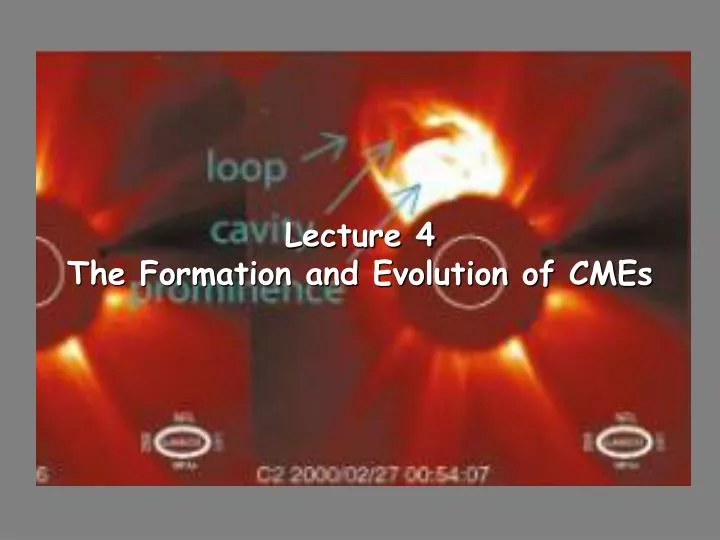
Lecture 4 The Formation and Evolution of CMEs. Coronal Mass Ejections (CMEs). Appear as loop like features that breakup helmet streamers in the corona. Three part structure: Bright outer rim Dark cavity behind rim Bright inner core of erupted prominence material. Scales of CMEs.

E N D
Coronal Mass Ejections (CMEs) • Appear as loop like features that breakup helmet streamers in the corona. • Three part structure: • Bright outer rim • Dark cavity behind rim • Bright inner core of erupted prominence material
Scales of CMEs • Gray areas are covered by codes • Micro – inertial length, Larmor radius • As CME propagates out through the solar system – both time and spatial scales increase (apparent shrinking is do to log log plot)
Prominences • Suspensions of cool (T~104K), dense (n~1010-1011 cm-3) chromospheric material surrounded by the hot (T~106K) and tenuous (n~107-109 cm-3) corona
Prominence Magnetic Field • Magnetic field is found to be approximately aligned with the filament. • Highly sheared field. • Called a filament when viewed from above. • Can be stable for days or weeks.
Fundamental Questions • How are CMEs initiated? • Widely accepted that the energy of CMEs is stored in coronal magnetic fields – the strongly sheared field of a filament (prominence) channel. • The CME is thought to be the catastrophic disruption of the force balance between the upward magnetic pressure of the filament and the downward tension of the overlying field. • How this disruption occurs is the main unanswered question in CME initiation. • Flux cancellation models • Breakout models • Flux injection model
Flux Cancellation Models • Flux cancellation is the disappearance of magnetic fields of opposite polarity at the neutral line separating them. • Flux cancellation at the neutral line of a sheared arcade causes the flux rope that supports prominence material. • Equilibrium breaks down if flux cancellation continues after the flux rope is formed. • A new equilibrium forms farther out. • In reality the solar wind pulls the flux rope out and forms a current sheet at which reconnection occurs.
A Simulation Study of the Eruption of a CME(Linker et al., 2003) • The initial configuration –azimuthal symmetry • Build a model of a helmet streamer • Use a spherically symmetric MHD solar wind solution • Use a potential magnetic field • Integrate until an equilibrium results. • To create a source of free magnetic energy put a shear flow near the neutral line of the streamer – specify the tangential E field.
Formation of a Flux Rope • (top) Projected field lines (shading) and azimuthal field (color) • (middle) Current density out of the plane. • (bottom) Polarization brightness that a coronagraph would observe. • Flux cancellation forms a stable flux rope within the helmet streamer (1350τA) • Once the configuration is beyond a stability threshold halting the flux cancellation cannot stop the eruption (1390τA). • Prominence formation is part of the flux cancellation mechanism.
Change in Magnetic Energy and Kinetic Energy • Magnetic energy closed flux (top-bottom), kinetic energy (bottom) • During formation of helmet streamer B2/2μ0 increases 15% (t<600) • Energization of streamer (600>t>1300) • Flux rope formation (1320) • Eruption (1380) • Energy of open flux (top-top) – eruption occurs when closed energy ~ open energy • Half of energy goes into flux rope.
Add azimuthal asymmetry • Azimuthal models – entire coronal field must be opened and flux rope is detached from the Sun. • 3D model allows azimuthal asymmetry. • Reduce magnetic flux only in one sector of Sun. • Creation of flux rope and eruption occur as before.
Structure of flux rope • Isosurface of density • Field lines in flux rope after it has propagated away from the Sun • Note that both ends of the flux rope are attached to the Sun.
The Breakout Model • Reconnection occurs external to the filament channel –quasi-potential overlying flux and neighboring flux systems. • Axisymmetric system with two spatial dimensions and three velocity dimensions (MacNeice et al., 2004). • Imposed shear flow at the equatorial neutral line – generates a Bφwhich produces an upward magnetic pressure (50251s, 70680s) • As fluxrope expands outward – downward tension on overlying field lines increases – stretch radially the field near the null. • Reconnection begins at the top of the expanding rope (79008) • Vertical current sheet forms deep inside (85185) – reconnects.
0 50251s 70680s 79008s 85185s 95020s
The Breakout Model and Observations • The main feature of the breakout model • “Flare” reconnection does not initiate the eruption, • Multipolar pre-eruption topology • Density difference shows changes in density. • The three part structure seen in coronagraph images is found in the simulations. Lynch et al., 2004
Energetics of the Breakout Model • Azimuthal magnetic energy – solid line • Azimuthal magnetic energy below 1.5RS – dashed-dotted line • Change in non-azimuthal energy – dashed line • The kinetic energy – dotted line with triangles. • Initially about half of the azimuthal magnetic energy is converted into kinetic energy. By the end of the simulation all magnetic energy about 1.5RS has been converted.
Flux Injection Model (Chen, 1989, 1996) • The underlying magnetic field of a CME is that of a three-dimensional flux rope. • While all models end up with flux ropes this one starts with them. • The flux rope is determined by the Lorentz force, pressure gradients and drag on the coronal plasma. • It is difficult to distinguish between the flux cancellation models and the flux injection model since they evolve in the same way once the flux rope emerges.
CME Evolution and Propagation (Forbes et al., 2006) • A CME propagates through the interplanetary medium as an ICME. • Assume a flux tube (the CME) circles the Sun like in the symmetric simulation. • Under excess internal pressure the flux tube expands – that expansion is resisted by the inertial reaction of the medium into which it expands. • The excess total pressure (particle plus magnetic) causes the flux tube to accelerate into the medium over coming gravity and drag.
Basic Interaction • The interaction can be written in words • Expansion • (Ambient mass density) X (Rate of expansion)2= Delta Pressure (inside – outside) • Acceleration • (Mass of CME + Virtual mass) X Acceleration = Force of gravity + Delta (outside magnetic and particle pressure on lower surface area – outside magnetic and particle pressure on upper surface area) – Drag • Virtual mass allows us to correct for the force necessary to move all the ambient medium away = volume of cylinder time the mass density of the ambient medium. • Problem is in turning this into equations. • Standard drag term CDAρ abs (VCME –Vsw) (VCME –Vsw) where CD is a drag coefficient, and (VCME –Vsw) is relative velocities of CME and solar wind. • How to do it is controversial.
MHD simulation of CME propagation in the heliosphere (Riley et al., 2003) • Combined a CME eruption model (flux cancellation) with a solar wind model. • Flux cancellation model was used as input to solar wind model. • Flux cancellation model assumes g=1.05 to mimic near-isothermal corona. • Solar wind model has g=5/3. • Discontinuity at interface is “harmless” affecting only temperature slightly. • Corotation enforced at the boundary between the models • Plasma and magnetic field parameters were set at the outer boundary of the heliospheric simulation
Evolution of the CME out to 0.5AU • Number density – black; Vr – color contours; Magnetic field lines – blue • White line is boundary between solutions. • Flux rope becomes circular and then “pancake” shaped – kinematic expansion as ejecta expands and then collision with surrounding material. • Shock and flux rope develop concave deformations.
Evolution of CME out to 5AU • Density – red, field lines – black and velocity shading. • Ejecta becomes more distorted with distance. • Acceleration related to post eruption reconnection.
Comparison with spacecraft observations • Ejecta was traveling faster than ambient solar wind –shock (both) • Speed profiles are similar • Simulated B does not have peak in sheath (ACE)) • Magnetic discontinuity not found in simulation (Ulysses) • B modeled better at Ulysses. • Strong magnetic structure at Ulysses but not at ACE – Ulysses passed near center of flux rope – ACE near the flank