Download
1 / 15
150 likes | 157 Views
Unified approach to the classical statistical analysis of small signals. Gary J. Feldman and Robert D. Cousins. Statistical Methods and Notation. Frequentist - P(x 0 | t ) Bayesian - P( t | x 0 ) - needs subjective P( t ) Feldman and Cousins use a frequentist (classical) model

E N D
Unified approach to the classical statistical analysis of small signals Gary J. Feldman and Robert D. Cousins
Statistical Methods and Notation • Frequentist - P(x0 | t) • Bayesian - P(t | x0) - needs subjective P(t) • Feldman and Cousins use a frequentist (classical) model • Confidence interval - [1,2] • A percentage (typically 90%) of all attempts to measure the value will give a value in this range
Confidence Belt FIG. 1. A generic confidence belt construction and its use. For each value of m, one draws a horizontal acceptance interval [x1 ,x2] such that P(x [x1 ,x2]|) = . Upon performing an experiment to measure x and obtaining the value x0, one draws the dashed vertical line through x0 . The confidence interval [m1 ,m2] is the union of all values of m for which the corresponding acceptance interval is intercepted by the vertical line.
Gaussian Curve y = 1/sqrt(2)*exp(-x2/2)
Gaussian FIG. 2. Standard confidence belt for 90% C.L. upper limits for the mean of a Gaussian, in units of the rms deviation. The second line in the belt is at x = +. FIG. 3. Standard confidence belt for 90% C.L. central confidence intervals for the mean of a Gaussian, in units of the rms deviation.
FIG. 4. Plot of confidence belts implicitly used for 90% C.L. confidence intervals (vertical intervals between the belts) quoted by flip-flopping physicist X, described in the text. They are not valid confidence belts, since they can cover the true value at a frequency less than the stated confidence level. For 1.36<<4.28, the coverage (probability contained in the horizontal acceptance interval) Is 85%.
Poisson Distribution FIG. 5. Standard confidence belt for 90% C.L. upper limits, for unknown Poisson signal mean m in the presence of a Poisson background with known mean b=3.0. The second line in the belt is at n=+. FIG. 6. Standard confidence belt for 90% C.L. central confidence intervals, for unknown Poisson signal mean m in the presence of a Poisson background with known mean b=3.0.
Solves Null Set problem FIG. 7. Confidence belt based on our ordering principle, for 90% C.L. confidence intervals for unknown Poisson signal mean m in the presence of a Poisson background with known mean b=3.0.
Background FIG. 9. Lower end m1 of our 90% C.L. confidence intervals [m1 ,m2], for unknown Poisson signal mean m in the presence of an expected Poisson background with known mean b. The curves correspond to the dotted regions in the plots of m2 of the previous figure, with again n0=10 for the upper right curve, etc. FIG. 8. Upper end m2 of our 90% C.L. confidence intervals [m1 , m2], for unknown Poisson signal mean m in the presence of an expected Poisson background with known mean b. The curves for the cases n0 from 0 through 10 are plotted. Dotted portions on the upper left indicate regions where m1 is non-zero ~and shown in the following figure!. Dashed portions in the lower right indicate regions where the probability of obtaining the number of events observed or fewer is less than 1%, even if m=0.
Gaussian Application FIG. 10. Plot of our 90% confidence intervals for the mean of a Gaussian, constrained to be non-negative, described in the text.
Fewer Events than Predicted Background • A good experiment could get a worse upper limit than a bad one if the predicted background was greater • Define new term - “sensitivity” • Upper limit that would be obtained by an ensemble of experiments with the expected background and no true signal
Sensitivity FIG. 15. Comparison of the confidence region for an example of the toy model in which sin2(2)=0 and the sensitivity of the experiment, as defined in the text.
Goodness of fit • Decouples confidence interval from goodness-of-fit C.L. • Standard classical intervals can give empty sets for confidence interval • Gaussian: if = 0, then 10% of the time, the empty set is obtained • This is equivalent to a failed goodness of fit
Feldman Cousins Approach • Unified approach - no distinct choices on whether to use an upper limit of central limit • Solves under-coverage problem (85%, when stated 90%) • Cost of a little over-coverage