Download

1 / 57
570 likes | 736 Views
Toby Walsh National ICT Australia and University of New South Wales www.cse.unsw.edu.au/~tw/global/. Global Constraints . Course outline. Introduction All Different Lex ordering Value precedence Complexity GAC-Schema Soft Global Constraints Global Grammar Constraints Roots Constraint

E N D
Toby Walsh National ICT Australia and University of New South Wales www.cse.unsw.edu.au/~tw/global/ Global Constraints
Course outline • Introduction • All Different • Lex ordering • Value precedence • Complexity • GAC-Schema • Soft Global Constraints • Global Grammar Constraints • Roots Constraint • Range Constraint • Slide Constraint • Global Constraints on Sets
Lex ordering • Widely useful • Especially for symmetry breaking • Breaking row and column symmetry in matrix models • Available in most (all?) solvers • Good example of pointer based global constraint • Pointers save re-doing work • Good incremental behaviour • O(n) in general, but amortised O(1) cost at each node down a branch
Motivation • Many problems can be modelled by matrices of decision variables.
Motivation • Many problems can be modelled by matrices of decision variables. • E.g. Combinatorial Problems • Balanced Incomplete Block Design. 0 1 1 0 0 1 0 1 0 1 0 1 0 0 0 0 1 1 0 0 1 1 1 0 0 0 0 1 <7,7,3,3,1> 0 0 0 0 1 1 1 1 0 0 1 0 1 0 0 1 0 1 1 0 0
Motivation • Many problems can be modelled by matrices of decision variables. • E.g. Configuration Problems: • Rack Configuration • Matrix is Xij iff jth card on ith rack
Motivation • Many problems can be modelled by matrices of decision variables. • E.g. Scheduling Problems: • Social Golfers • 32 golfers want to play in 8 foursomes each day of the week • No two golfers shall meet twice in a foursome • Matrix is Pijk=1 iff player i plays in jth foursome on day k
Motivation • Many problems can be modelled by matrices of decision variables. • E.g. Design Problems: • Steel Mill Slab Design • Slab[o,j] iff order o is on jth slab • IBM solved this problem for the largest steel maker in Korea
Motivation • Many problems can be modelled by matrices of decision variables. • Frequently these matrices exhibit row and/or column symmetry.
Motivation • Many problems can be modelled by matrices of decision variables. • Frequently these matrices exhibit row and/or column symmetry. • We can permute the rows/columns in any (non)solution to obtain another (non)solution.
Motivation • An important class of symmetries in CP • matrices of decision variables • rows/columns represent indistinguishable objects, hence symmetric • Rows and columns are subject to permutation • An nXm matrix model with row and column symmetry has n! Xm! symmetries • grows super-exponentially • Too many symmetric search states • It can be very expensive to visit all the symmetric branches of a search tree
Motivation • Breaking symmetry is very important! • Breaking all row and column symmetries is difficult • No one has an effective way of dealing with all row and column symmetries. • Symmetry breaking methods have to deal with very large number of symmetries. • The effort required could easily be exponential.
Frequently occurs Combinatorial problems like covering arrays Rows and columns can be permuted Messy real world problems like nurse rostering Nurses with same skills can be swapped Tough for IP Very active research area within CP Some effective techniques have been developed Symmetry
Modelling adds symmetry • Divide 32 golfers into 8 foursomes so that each week they play with different players • Xijk = ith player in jth group in kth week • In this model, we can permute • players within group • groups • weeks Representing a set like a foursome by 4 variables, introduces symmetries (their permutations)! Social golfers problem
Symmetry in CP • Add symmetry breaking constraints • Leave at least one solution • Eliminate some/all symmetric solutions • Modify search algorithm • Ignore symmetric parts of the search space • Adapt branching heuristic • To explore branches which are most likely not to be symmetric
Example • Consider 2 identical bins: A B
Example • Consider 2 identical bins: A B • We must pack 6 items: 1 2 3 4 5 6
Example • Here is one solution: 5 6 3 4 1 2 A B
Example • Here is another: 6 5 4 3 2 1 A B
Example • Is there any fundamental difference? 5 6 a) 3 4 1 2 A B 6 5 b) 4 3 2 1 A B
Example • Consider a matrix model: 5 6 a) 3 4 1 2 A B 6 5 b) 4 3 2 1 A B
Example • Consider a matrix model: 1 2 3 4 5 6 A 1 0 1 0 1 0 B 0 1 0 1 0 1 5 6 a) 3 4 1 2 A B 1 2 3 4 5 6 A 0 1 0 1 0 1 B 1 0 1 0 1 0 6 5 b) 4 3 2 1 A B
If we insist that row A lex row B, we remove a) from the solution set. Example • Consider a matrix model: 1 2 3 4 5 6 A 1 0 1 0 1 0 B 0 1 0 1 0 1 1 2 3 4 5 6 A 0 1 0 1 0 1 B 1 0 1 0 1 0 6 5 b) 4 3 2 1 A B
Example • Notice that items 3 and 4 are identical. 1 2 3 4 5 6 A 1 0 1 0 1 0 B 0 1 0 1 0 1 6 5 b) 4 3 2 1 A B 1 2 3 4 5 6 A 0 1 1 0 0 1 B 1 0 0 1 1 0 6 5 c) 3 4 2 1
If we insist that col 3 lex col 4, we remove c) from the solution set. Example • Notice that items 3 and 4 are identical. 1 2 3 4 5 6 A 1 0 1 0 1 0 B 0 1 0 1 0 1 6 5 b) 4 3 2 1 A B 1 2 3 4 5 6 A 0 1 1 0 0 1 B 1 0 0 1 1 0
Lexicographic Ordering • Used to order dictionaries [A,B,C] ≤ lex [D,E,F] • A<D or • (A=D and B<E ) or • (A=D and B=E and C<F) or • (A=D and B=E and C=F)
Breaking Row (Column) Symmetry • Lexicographic ordering is total • Forcing the rows to be lexicographically ordered breaks all row symmetry • anti-lexicographic ordering • lexicographic ordering • [A B C] lex [D E F] lex [G H I] • [G H I] lex [D E F] lex [A B C]
Breaking Row and Column Symmetries • Breaking both row and column symmetries is difficult • Rows and columns intersect • After constraining the rows to be lexicographically ordered • we distinguish the columns • the columns are not symmetric anymore!
Each symmetry class of assignments has at least one element where both the rows and the columns are lexicographically ordered But there may be no element with rows lex ordered and columns anti-lex ordered To break row and column symmetries, we can insist that the rows and columns are both lexicographically ordered (double-lex) Extends to higher dimensions Good News
Bad News • A symmetry class of assignments may have more than one element where both the rows and the columns are lexicographically ordered • Double-lex does not break all row and column symmetries 0 1 0 1 0 1 1 0 swap the columns swap row 1 and row 3 1 0 1 0
Special Cases • All symmetry can be broken • When variables take distinct values • Simply push largest value to a particular corner • Order 1st row and 1st col • 0/1 variables, 1 occurs once in each row/col • Double LEX then leaves an unique solution
GACLex • A new family of global constraints.
GACLex • A new family of global constraints. Non-binary constraint. Specialised propagator.
GACLex • A new family of global constraints. • Linear time complexity.
GACLex • A new family of global constraints. • Linear time complexity. • Ensures that a pair of vectors of variables are lexicographically ordered. lex
How GACLex Works • Consider the following example. • We have two vectors of decision variables: • We want to enforce GAC on: xlexy.
A Tale of Two Pointers • We use two pointers, alpha and beta, to avoid repeatedly traversing the vectors
A Tale of Two Pointers Most significant index
A Tale of Two Pointers • alpha: index such that all variables at more significant indices are ground and equal.
A Tale of Two Pointers • We use two pointers, alpha and beta, to avoid repeatedly traversing the vectors. • beta: most significant index from which the two vectors’ tails necessarily violate the constraint.
Pointer initialization • alpha • Scan through vector from start • At most O(n) time • beta • Scan through vector from end • At most O(n) time
Failure • Inconsistent if betaalpha. • alpha: index such that all variables at more significant indices are ground and equal. • beta: most significant index from which the two vectors’ tails necessarily violate the constraint.
How GACLex Works • We maintain alpha and beta as assignments made. • alpha: index such that all variables at more significant indices are ground and equal. • beta: most significant index from which the two vectors’ tails necessarily violate the constraint.
How GACLex Wroks • We maintain alpha and beta as assignments made. • When beta = alpha + 1 we enforce bounds consistency on: xalpha < yalpha • alpha: index such that all variables at more significant indices are ground and equal. • beta: most significant index from which the two vectors’ tails necessarily violate the constraint.
How GACLex Works • We maintain alpha and beta as assignments made. • When beta = alpha + 1 we enforce bounds consistency on: xalpha < yalpha • When beta > alpha + 1 we enforce bounds consistency on: xalphayalpha • alpha: index such that all variables at more significant indices are ground and equal. • beta: most significant index from which the two vectors’ tails necessarily violate the constraint.
Complexity • Initialisation: O(n) • Propagation: • We enforce bounds consistency between at most n pairs of variables: xalpha < yαalpha or xalphayαalpha. • Cost: b. Overall cost: O(nb).
Why Have a Global LEX Constraint? • Two alternatives • Arithmetic constraint • Logical decomposition • Both limit problem size • And both can be slower! • Both do less pruning than GAC(X0<lex X1 <lex ... <lex Xn)
Arithmetic Constraint • Given A=[a1,...,an] B=[b1,...,bn] taking values from {1,...d} A≤lexB iff(dn-1a1+ ... + d0an) ≤ (dn-1b1+ ... + d0bn) • BC(≤) iff GAC(≤lex) • When n and d are large, dn-1 is greater than the word size of the computer. • This method is only feasible for small vectors/domain size.
Many solvers use FC Less pruning than GAC GAC schema is expensive They are also cumbersome. Logical Decompositions • Or decomposition A≤lexB iff (a1 < b1) Or (a1 = b1 And a2 < b2 ) ... (a1 = b1 And a2 = b2 ... an ≤ bn) • And decomposition A≤lexB iff (a1 ≤ b1) And (a1 = b1 -> a2 ≤ b2 ) ... (a1 = b1 And a2 = b2 ... -> an ≤ bn)