GG 313 Geological Data Analysis Lecture 13 Solution of Simultaneous Equations October 4, 2005

1. GG 313 Geological Data Analysis Lecture 13 Solution of Simultaneous Equations October 4, 2005

2. Homework discussion. People are having problems with the null hypothesis and what the solution to a hypothesis test means. Rejecting the null hypothesis is the positive result of our tests. We need to understand what this means, and the easiest way is by example.

3. Consider the Mann-Whitney Test and example 2-7 (page 45). Comparing grain sizes from two different locations on the moon, we want to see if the mean grain sizes differ in the two samples. Of course they won’t be the same, but is the difference statistically significant? Our hypothesis is that the the mean grain size is different, implying the two samples come from different populations. Our null hypothesis is thus that the mean grain sizes are the same with some statistical confidence (95%). In this test we combine the two samples and rank eache element of the sample. If the two samples were identical, then they would have the same W1 and W2, which would be (eqn. 2.33) and U1 and U2 would equal zero.

4. Since U=0 is certainly less than the critical value (U) obtained from the table. So as U increases, the two means are getting farther apart. We cannot disprove our null hypothesis if U is smaller than U. In the notes for this example, U=24 and U=20. So we can conclude that the two means cannot be the same with 95% certainty. IN THE NOTES, Paul says “This (U=24) is larger than the critical value of 20, suggesting we cannot reject the null hypothesis.” He’s wrong. Don’t believe everything you read. Another example: Homework 5, problem 1. It states: “… do these data support the claim that on average higher concentrations were obtained before cleaning versus after cleaning?” What is the hypothesis?

5. What is the null hypothesis? • These data are in PAIRS. We are trying to figure out if the “before” number is statistically larger than the “after” number. • Using the “sign” test, what do you do first? • subtract the 2nd number of each pair from the first. If the first is larger, the result will be “+”, if the first is smaller, the result will be “-”. How many “+” are there? • If there were as many + as -, what would that say about the null hypothesis? • If the number of + is much larger than the number of -, what would that say?

6. You can calculate the probability of having n + using the binomial coefficients, but that’s a lot of work. Since, for this problem, np>5 and n(1-p)>5, you can use z-statistics (eqn. 2.32). If your z-value from the data is >2, what does that mean? These tests are not difficult, but you do need to think the logic through. You cannot expect to blindly use the notes and formulas and come up with the correct answer. Since there’s a 50% probability that you’ll get the answer right, the method is everything.

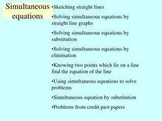
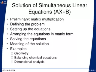
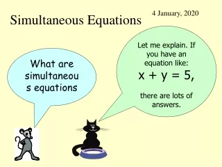
7. Linear algebra provides us with an easy method for solving systems of simultaneous equations. Consider the following set of four equations with four unknowns x1,x2,x3,and x4: (3.77) In matrix form, the above is just:

8. Where: (3.79-3.81) The solution to the equations is obtained by multiplying both sides of Eqn. 3.78 by A-1, to obtain: (3.82) (3.83)

9. We have thus solved for x and obtained the solution. EXAMPLE: Consider a simple example. We have three planes that are defined below. Any three planes cross at a point. At what point do they cross each other? x-y-2z=2 x+y+2z=10 -2x-2y-z=3 Setting up the matrix:

10. In Matlab: >> Ainv=inv(A) Ainv = 0.5000 0.5000 0 -0.5000 -0.8333 -0.6667 0 0.6667 0.3333 Multiplying by B, >> X=Ainv*B X = 6.0000 =x -11.3333 =y 7.6667 =z Thus the planes cross at the point above.

11. I think this is an easy way to solve such sets of equations, particularly as the number of equations and unknowns increase. Other methods may be computationally more efficient, but the above method is easy to set up and solve. _______________ Try an example where you know the answer: Try the x-z plane at y=2 (0x+1y+0z=2), the x-y plane at z=0 (0x+0y+1z=0), and the y-z plane at x=-2 (1x+0y+0z=-2). Where do these 3 planes cross? Solve graphically and using the matrix solution.

12. Solutions of this sort are relatively simple. We have no options - there is only one correct answer and no freedom to choose between possible answers. A more interesting case is where we have more data than we need to fit a model. For example, as we’ve said before, two points define a line. But what if we want to define a line a line with three points? A and B define a line, but added data (point C) sheds doubt on our original interpretation.

13. We would like to define a new line that is somehow the “best” line given the data we have. In addition, we would like to know just how likely it is that the new line, which is an estimate based on a sample of all points in the population, reflects the population. We must be careful! We are assuming that our MODEL (a straight line) reflects the shape of reality. A “best fit” does not validate the model. A good bet for finding the “best” fit to a model curve is to minimize the square of the errors of each point with respect to the model curve. Thus, we want to find the curve that minimizes these errors: This figure works well, but what if the line is nearly vertical?

14. The figure above shows the errors in the y-value (regression of y on x). Similarly, we could find the errors in x: Do these two methods yield the same answers? Consider the case below: In this case the errors in y are far smaller than the errors in x, and utilizing errors in y will likely yield a better result. If the curve had a steep slope, the opposite would be the case.

15. In any case, we can use a method that does not vary with slope of the curve by measuring perpendiculars to the curve at each point: This method, called orthogonal regression, is most useful when the slope of the line is unknown and it can be in any direction.

16. We wish to find a line of the form: y(x)=a1+a2(x-x0). (3.89) Why does Paul use x0? Note that y(x)=a1+a2x-a2x0, so y(x)=(a1-a2x0)+a2x=a3+a2x. So why bother with x0??? Let’s ignore it… We have two unknowns, a1and a2, and we wnt to find values of these unknowns that minimize the square of the error: (3.90)

17. We have one equation for each data point: (3.91) We only need two equations to solve for a1 and a2, but we have n equations. This situation is called over-determined. The only way these equations can have a unique solution is for n to equal 2 or if all the points lie exactly on a straight line.

18. A x=b : We can write the equations in matrix notation, (3.92) Why can’t we just invert as we did before, and solve for x=A-1b ? Unfortunately, this isn’t possible since A isn’t square, and it thus has no inverse. But all is not lost… Consider the equations:

19. (3.93) ei is the error of the observed y minus the theoretical value, and we want to obtain the values of a1 and a2 that minimize the sum of the squares of the ei: (3.94) Recall the definition of variance. Minimization of E will minimize the variance of the errors. Recall that if E is minimum then the slope of E must be equal to zero.

20. E is a function of two variables, and the slope must be zero for each, which says: (3.95) Evaluating: (3.96) (3.97)

21. With the results from the two equations (3.96 and 3.97) we have two equations and two unknowns (a1 and a2), and we can solve. Re-arranging: (3.98) (3.99) Note that the unknowns are a1 and a2, and that the x and y values are known, so the sumations in the equations above are all of known constants. We form the sums as follows (notation is poor here; S stands for sum, not covariance): (3.100)

22. Substituting: 3.101 3.102 Solving for the y-intercept, a1 in the first equation, 3.103 Substituting into the first equation for a1 yields: 3.107

23. In matrix notation: (3.109) This matrix is of the form N x = B, which can be solved for x by x = N-1 B.

24. In - class problem: Use the following data and calculate the least-squares fit to a line using eqn. 3.109. Data points: x y -33 -5 -2 50 -44