Download
1 / 32
320 likes | 880 Views
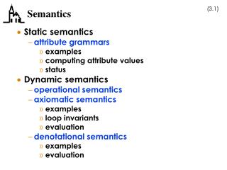
Semantics. “Semantics” has to do with the meaning of a program. We will consider two types of semantics: Static semantics: semantics which can be enforced at compile-time. Dynamic semantics: semantics which express the run-time meaning of programs. Static semantics.

E N D
Semantics • “Semantics” has to do with the meaning of a program. • We will consider two types of semantics: • Static semantics: semantics which can be enforced at compile-time. • Dynamic semantics: semantics which express the run-time meaning of programs.
Static semantics • Semantic checking which can be done at compile-time • Type-compatibility • int can be assigned to double (type coercion) • double cannot be assigned to int without explicit type cast • Can be captured in grammar, but only at expense of larger, more complex grammar
Type rules in grammar • Must introduce new non-terminals which encode types: • Instead of a generic grammar rule for assignment: • <stmt> <var> ‘=’ <expr> ‘;’ • we need multiple rules: • <stmt> <doubleVar> ‘=’ <intExpr> | <doubleExpr> ‘;’ • <stmt> <intVar>‘=’ <intExpr> ‘;’ • Of course, such rules need to handle all the relevant type possibilities (e.g. byte, char, short, int, long, float and double).
Attribute grammars • Attribute grammars provide a neater way of encoding such information. • Each syntactic rule of the grammar can be decorated with: • a set of semantic rules/functions • a set of semantic predicates
Attributes • We can associate with each symbol X of the grammar a set of attributes A(X). Attributes are partitioned into: synthesized attributes S(X) – pass info up parse tree inherited attributes I(X) – pass info down parse tree
Semantic rules/functions • We can associate with each rule R of the grammar a set of semantic functions. • For rule X0 X1 X2 … Xn • synthesized attribute of LHS: S(X0) = f(A(X1), A(X2), …, A(Xn)) • inherited attribute of RHS member: for 1<=j<=n, I(Xj) = f(A(X0),…,A(Xj-1)) (note that dependence is on siblings to left only)
Predicates • We can associate with each rule R of the grammar a set of semantic predicates. • Boolean expression involving the attributes and a set of attribute values • If true, node is ok • If false, node violates a semantic rule
Example <assign> <var> = <expr> <expr>.expType <var>.actType <expr> <var>[2] + <var>[3] <expr>.actType if (var[2].actType = int) and (var[3].actType = int) then int else real <expr>.actType == <expr>.expType <expr> <var> <expr>.actType <var>.actType <expr>.actType == <expr>.expType <var> A | B | C <var>.actType lookUp(<var>.string) Syntactic rule Semantic rule/function Semantic predicate
<assign> <expr> <var> <var>[2] <var>[3] Suppose: A is int B is int A = A + B
<assign> expected type = int actual type = int <expr> actual type = int <var> <var>[2] <var>[3] actual type = int actual type = int actual type = int Suppose: A is int B is int A = A + B
<assign> expected type = real actual type = real type coercion during ‘+’: int real <expr> actual type = real <var> <var>[2] <var>[3] actual type = real actual type = int actual type = real Suppose: A is real B is int A = A + B
<assign> Houston, we have a problem! Semantic predicate is false. expected type = int actual type = real <expr> actual type = int <var> <var>[2] <var>[3] actual type = int actual type = real actual type = int Suppose: A is int B is real A = A + B
Dynamic semantics • Dynamic semantics precisely specify the meanings of programs. • Why is this important? • programmers need to understand the meanings of programs they read • programmers need to understand how to express themselves in a given language • compiler writers need to understand how to translate a high-level program into a semantically equivalent low-level one • Formal semantics are not always used – no single formalism exists. We will look at: • operational semantics • axiomatic semantics • There is also denotational semantics. Look in text if you’re interested.
Operational semantics • Basic idea: we describe the meanings of program elements by describing how a machine executes them. • Basic approach: express semantics of a high-level construct in terms of its translation into a low-level construct • Example: Java described in terms of JVM • Example: Pascal described in terms of p-code • Example: C described in terms of PDP-11 assembly
Examplehigh-level programoperational semantics for (e1; e2; e3) { . . . } <rest of program> e1; L1: if not(e2) goto L2 . . . e3; goto L1 L2: <rest of program>
Axiomatic semantics • Basic idea: you make assertions about statements in a program. • A precondition is an assertion about what is true prior to execution of a statement. • A postcondition is an assertion about what is true after execution of a statement. For example: sum = 2*sum + 1 {sum > 1}
Weakest precondition • “The weakest precondition is the least restrictive precondition that will guarantee the validity of the associated postcondition.” [p. 151] • In example above {sum>10} is a valid precondition but {sum>0} is the weakest precondition: {sum > 0} sum = 2*sum + 1 {sum > 1}
Correctness proofs • “If the weakest precondition can be computed from the given postconditions for each statement of a language, then correctness proofs can be constructed for programs in that language.” [p. 151] • To do this, start with output specifications for the program as the postcondition for the program as a whole.
Next, work backwards, computing weakest preconditions one statement at a time, to derive the weakest precondition for the program as a whole: stmt1 {c0} stmt1 {c1} stmt2 {c1} stmt2 {c2} . . . . . . stmtN {cN} {cN-1} stmtN {cN}
If the input specification for the program satisfies the program’s weakest precondition, then the program will (provably) produce the correct result.
Assignment statements • The axiomatic semantics of an assignment statement x=E is written as P=QxE • This means that the precondition is the postcondition with all instances of x replaced by E. • Example: a = b/2-1 {a<10} To compute precondition, replace all instances of a in postcondition a<10 by b/2–1: b/2-1 < 10, or b < 22 • Semantics: {b<22} a = b/2-1 {a<10} • In general: {QxE} x=E {Q}
Inference • Suppose we wanted to prove the following: {sum > 5} sum = 2*sum + 1 {sum > 3} • Starting with the postcondition, we derive as the weakest precondition something different: 2*sum + 1 > 3 2*sum > 2 sum > 1 (weakest precondition) • Clearly this is OK, because the actual precondition {sum>5} implies the weakest precondition {sum>1}: sum>5 => sum>1 • We use an inference rule, the rule of consequence, to prove this.
Rule of consequence • General form: S1, S2, …, Sn S • Precondition strengthening: P=>P’, {P’} C {Q} {P} C {Q} • Postcondition weakening: Q’=>Q, {P} C {Q’} {P} C {Q}
Precondition strengthening applied • Recall our example. We want to prove the following: {sum > 5} sum = 2*sum + 1 {sum > 3} • The weakest precondition we derive is: sum > 1 • Apply precondition strengthening to finish proof: P=>P’, {P’} C {Q} {P} C {Q} sum>5 => sum>1, {sum>1} sum=2*sum+1 {sum>3} {sum>5} sum=2*sum+1 {sum>3}
Hang on! • Why get so formal? • Because this way correctness proofs can be (partially) automated.
{P} S1 {Q}, {Q} S2 {R} • {P} S1 S2 {R} Sequences:S1 S2 Start with a sequence of statements: y = 3*x+1; x = y+3; {x<10} Compute weakest precondition for 2nd stmt: {y+3<10} or {y<7}, use as postcondition for 1st stmt: y = 3*x+1; {y<7} {y<7} x = y+3; {x<10} Compute weakest precondition for 1st stmt: {3x+1<7} or {x<2} {x<2} y = 3*x+1; {y<7} {y<7} x = y+3; {x<10} Conclude, applying sequence rule: {x<2} y = 3*x+1; x = y+3; {x<10}
{B & P} S1 {Q}, {!B & P} S2 {Q} • {P} if B then S1 else S2 {Q} Selection:if B then S1 else S2 Start with a conditional statement: if (x>0) then y=y-1 else y=y+1 {y>0} Deal with arms of the conditional one at a time, first the then-arm: y = y-1 {y>0} {y>1} y = y-1; {y>0} Now the else-arm: y = y+1 {y>0} {y>-1} y = y+1; {y>0} Use rule of precondition strengthening on the else-arm result (to make both arms uniform): {y>1} y = y+1; {y>0} Now strengthen both arms’ preconditions by imposing a constraint on x: { x>0 & y>1} y = y-1; {y>0} {!(x>0) & y>1} y = y+1; {y>0} Conclude, applying selection rule: {y>1} if (x>0) then y=y-1 else y=y+1 {y>0}
{B & I} S {I} _ • {I} while B do S end {I and !B} While:while B do S end Let’s prove the following: {true} r=x; q=0; while y<=r do r=r-y; q=q+1; end {y>r & x=r+y*q} Start by proving loop body: {y<=r & x=r+y*q} r=r-y; q=q+1;{x=r+y*q} Start with last statement: q=q+1 {x=r+y*q} {x=r+y*(q+1)} q=q+1 {x=r+y*q} {x=r+y+y*q} q=q+1 {x=r+y*q} Continue with second-to-last statement: r=r-y {x=r+y+y*q} {x=r-y+y+y*q} r=r-y {x=r+y+y*q} {x=r+y*q} r=r-y {x=r+y+y*q} Use rule for sequence to get: {x=r+y*q} r=r-y; q=q+1; {x=r+y*q} Now strengthen precondition to conclude proof of loop body: {y<=r & x=r+y*q} r=r-y; q=q+1; {x=r+y*q} This lets us derive a weakest precondition for the while loop: {x=r+y*q} while y<=r do r=r-y; q=q+1; end {x=r+y*q & !(y<=r)}
{B & I} S {I} _ • {I} while B do S end {I and !B} While:while B do S end The next step is to prove the sequence {true} r=x; q=0; while y<=r do r=r-y; q=q+1; end {x=r+y*q & y>r)} Start by moving backwards from the while loop (since we derived a weakest precondition from its postcondition already): {true} r=x; q=0; {x=r+y*q} Start with last statement: q=0; {x=r+y*q} {x=r+y*0} q=0 {x=r+y*q} {x=r} q=0 {x=r+y*q} Continue with second-to-last statement: r=x {x=r} {x=x} r=x {x=r} Precondition strengthening: {true} r=x {x=r} Sequence rule (applied in general form): {true} r=x; q=0; while y<=r do r=r-y; q=q+1; end {x=r+y*q & !(y<=r)} Finally, postcondition weakening because !(y<=r) => y>r : {true} r=x; q=0; while y<=r do r=r-y; q=q+1; end {x=r+y*q & y>r} We're done!
Loop invariant • Recall the While rule: {B & I} S {I} _ {I} while B do S end {I and !B} • I is called the loop invariant: • "…if executing [the body] once preserves the truth of [the invariant], then executing [the body] any number of times also preserves the truth of [the invariant]." [Gordon, Programming Language Theory and its Implementation, paraphrased from page 24]
Importance of loop invariants • Developing loop invariants are a powerful way to design and understand algorithms. • Consider selection sort: selectionSort(int[] array) { int min, temp, bar=0; while (bar < array.length - 1) { min = indexOfSmallest(array, bar); // find min temp = array[bar]; // swap array[bar] = array[min]; array[min] = temp; bar = bar + 1; // Loop invariant: region before bar is sorted // for all i,j<=bar, if i<j, array[i] <= array[j]} }
Example [ 7 4 6 8 3 2 ] [ 24 6 8 3 7 ] [ 2 36 8 4 7 ] [ 2 3 48 6 7 ] [ 2 3 4 68 7 ] [ 2 3 4 6 7 8 ] region not known to be sorted region known to be sorted