Download
1 / 26
280 likes | 506 Views
Bayesian Probabilistic or Weights of Evidence Model for Mineral Prospectivity Mapping. Probabilistic model (Weights of Evidence). What is needed for the WofE calculations? A training point layer – i.e. known mineral deposits; One or more predictor maps in raster format.

E N D
Bayesian Probabilistic or Weights of Evidence Model for Mineral Prospectivity Mapping
Probabilistic model (Weights of Evidence) • What is needed for the WofE calculations? • A training point layer – i.e. known mineral deposits; • One or more predictor maps in raster format.
PROBABILISTIC MODELS (Weights of Evidence or WofE) • Four steps: • Convert multiclass maps to binary maps • Calculation of prior probability • Calculate weights of evidence (conditional probability) for each predictor map • Combine weights
The probability of the occurrence of the targeted mineral deposit type when no other geological information about the area is available or considered. Calculation of Prior Probability 1k Study area (S) 1k Target deposits D • Assuming- • Unit cell size = 1 sq km • Each deposit occupies 1 unit cell 10k Total study area = Area (S) = 10 km x 10 km = 100 sq km = 100 unit cells Area where deposits are present = Area (D) = 10 unit cells Prior Probability of occurrence of deposits = P {D} = Area(D)/Area(S)= 10/100 = 0.1 Prior odds of occurrence of deposits = P{D}/(1-P{D}) = 0.1/0.9 = 0.11 10k
Convert multiclass maps into binary maps • Define a threshold value, use the threshold for reclassification Multiclass map Binary map
Convert multiclass maps into binary maps • How do we define the threshold? Use the distance at which there is maximum spatial association as the threshold !
Convert multiclass maps into binary maps • Spatial association – spatial correlation of deposit locations with geological feature. A A 10km D D C C B B 1km 10km 1km Study area (S) Gold Deposit (D)
Convert multiclass maps into binary maps Which polygon has the highest spatial association with D? More importantly, does any polygon has a positive spatial association with D ??? A Positive spatial association – more deposits in a polygon than you would expect if the deposits were randomly distributed. D C B What is the expecteddistribution of deposits in each polygon, assuming that they were randomly distributed? What is the observed distribution of deposits in each polygon? If observed >> expected; positive association If observed = expected; no association If observed << expected; negative association
Convert multiclass maps into binary maps OBSERVED DISTRIBUTION Area (A) = n(A) = 25; n(D|A) = 2 Area (B) = n(A) = 21; n(D|B) = 2 Area(C) = n(C) = 7; n(D|C) = 2 Area(D) = n(D) = 47; n(D|D) = 4 Area (S) = n(S) = 100; n(D) = 10 A D C B
Convert multiclass maps into binary maps EXPECTED DISTRIBUTION A Area (A) = n(A) = 25; n(D|A) = 2.5 Area (B) = n(A) = 21; n(D|B) = 2.1 Area(C) = n(C) = 7; n(D|C) = 0.7 Area(D) = n(D) = 47; n(D|D) = 4.7 (Area (S) = n(S) = 100; n(D) = 10) D C B Expected number of deposits in A = (Area (A)/Area(S))*Total number of deposits
Convert multiclass maps into binary maps EXPECTED DISTRIBUTION OBSERVED DISTRIBUTION Area (A) = n(A) = 25; n(D|A) = 2 Area (B) = n(A) = 21; n(D|B) = 2 Area(C) = n(C) = 7; n(D|C) = 2 Area(D) = n(D) = 47; n(D|D) = 4 Area (S) = n(S) = 100; n(D) = 10 Area (A) = n(A) = 25; n(D|A) = 2.5 Area (B) = n(A) = 21; n(D|B) = 2.1 Area(C) = n(C) = 7; n(D|C) = 0.7 Area(D) = n(D) = 47; n(D|D) = 4.7 (Area (S) = n(S) = 100; n(D) = 10) A Only C has positive association! So, A, B and D are classified as 0; C is classified as 1. D • Another way of calculating the spatial association : • = Observed proportion of deposits/ Expected proportion of deposits • = Proportion of deposits in the polygon/Proportion of the area of the polygon • = [n(D|A)/n(D)]/[n(A)/n(S)] • Positive if this ratio >1 • Nil if this ratio = 1 • Negative if this ratio is < 1 C B
Convert multiclass maps into binary maps – Line features A L 10km D C B 1km 10km 1km Study area (S) Gold Deposit (D)
Convert multiclass maps into binary maps – Line features 1 1 2 3 4 5 6 7 8 9 1 0 2 3 4 5 6 7 8 1 1 1 0 2 3 4 5 6 7 8 2 1 2 3 4 5 6 7 0 1 0 3 2 1 2 3 4 5 6 1 3 2 1 1 0 2 3 4 5 6 4 3 2 1 1 0 2 3 4 5 4 3 2 1 1 1 2 3 4 0 5 4 3 2 0 1 1 2 3 4 1km 1 0 5 4 3 2 1 2 3 4 1km Gold Deposit (D)
Convert multiclass maps into binary maps – Line features • Calculate observed vs expected distribution of deposits for cumulative distances 1 1 2 3 4 5 6 7 8 9 1 0 2 3 4 5 6 7 8 1 1 1 0 2 3 4 5 6 7 8 2 1 2 3 4 5 6 7 0 1 0 3 2 1 2 3 4 5 6 1 3 2 1 1 0 2 3 4 5 6 4 3 2 1 1 0 2 3 4 5 4 3 2 1 1 1 2 3 4 0 5 4 3 2 0 1 1 2 3 4 1 0 5 4 3 2 1 2 3 4 Gold Deposit (D) =< 1 – positive association (Reclassified into 1) >1 – negative association (Reclassified into 0)
1k 1k Unit cell Target deposits Geological Feature (B1) Geological Feature (B2) Calculation of Weights of Evidence Weights of evidence ~ quantified spatial associations of deposits with geological features Study area (S) 10k 10k Objective: To estimate the probability of occurrence of D in each unit cell of the study area Approach: Use BAYES’ THEOREM for updating the prior probability of the occurrence of mineral deposit to posterior probability based on the conditional probabilities (or weights of evidence) of the geological features.
Observation Inference P{D& B} P{B|D} Posterior probability of D given the presence of B • P{D|B} = = P{D} P{B} P{B} P{D & B} P{B|D} • P{D|B} = Posterior probability of D given the absence of B = P{D} P{B} P{B} Calculation of Weights of Evidence D- Deposit B- Geol. Feature Bayes’ theorem: THE BAYES EQUATION ESTIMATES THE PROBABILTY OF A DEPOSIT GIVEN THE GEOLOGICAL FEATURE FROM THE PROBABILITY OF THE FEATURE GIVEN THE DEPOSITS
It has been observed that on an average 100 gold deposits occur in 10,000 sq km area of specific geological areas. In such areas, 80% of deposits occur in Ultramafic(UM) rocks, however, 9.6% of barren areas also occur in Ultramafic rocks. You are exploring a 1 sq km area of an Archaean geological province with Ultramafic rocks (UM). What is the probability that the area will contain a gold deposit? Assume that a gold deposit occupies 1 sq km area. EXERCISE P(D|UM) = P(D) x [P(UM|D) / P(UM)] P(D) = n(D)/n(S) P(UM|D) = n(UM & D)/n(D) P(UM) = n(UM)/n(S) 10,000 n(S) = n(D) = n(UM&D) = n(UM) = n(UM) = P(D|UM) = (100/10000) * [(80/100)/(1030.4/10000)] = 0.077 100 80 ? 80% of 100 + 9.6% (10,000 - 100) = 1030.4
+ive weight of evidence (W+) -ive weight of evidence (W-) Calculation of Weights of Evidence Using odds (P/(1-P)) formulation: P{B|D} • O{D|B} = Odds of D given the presence of B O{D} P{B|D} P{B|D} • O{D|B} = Odds of D given the absence of B O{D} P{B|D} Taking logs on both sides: P{B|D} • Loge (O{D|B}) = Log of odds of D given the presence of B Loge(O{D}) + loge P{B|D} P{B|D} • Loge (O{D|B}) = Log of odds of D given the absence of B Loge(O{D}) + loge P{B|D}
Contrast (C) measures the net strength of spatial association between the geological feature and mineral deposits Contrast = W+ – W- + ive Contrast – net positive spatial association -ive Contrast – net negative spatial association zero Contrast – no spatial association Can be used to test spatial associations Calculation of contrast
B1 D B1 D B1 D B1 D Calculation of Probabilty B1 B2 P(D) = n(D)/n(S) = n( )/n(D) = n( )/ = n( )/n(D) = n( )/ D B & D P{B|D} P{B|D} n(D) B & D P{B|D} B & D P{B|D} n(D) B & D S B1 D Total number of cells in study area: n(S) Total number of cells occupied by deposits (D): n(D) Total number of cells occupied by the feature (B): n(B) Total number of cells occupied by both feature and deposit: n(B&D)
P{B|D} W- = loge P{B|D} B1 D B1 D B2 D B2 D B1 D B2 D B1 D B2 D P{B|D} P{B|D} Calculation of Weights of Evidence B1 loge W+ = B2 = n( )/n(D) = n( )/ = n( )/n(D) = n( )/ D Where, B & D P{B|D} P{B|D} n(D) B & D P{B|D} B & D P{B|D} n(D) B & D S B1 D Probabilities are estimated as area (or no. of unit cells) proportions Basic quantities for estimating weights of evidence Total number of cells in study area: n(S) Total number of cells occupied by deposits (D): n(D) Total number of cells occupied by the feature (B): n(B) Total number of cells occupied by both feature and deposit: n(B&D) S B2 D Derivative quantities for estimating weights of evidence D Total number of cells not occupied by D: n( ) = n(S) – n(D) Total number of cells not occupied by B: n( ) = n(S) – n(B) Total number of cells occupied by B but not D: n( B & D) = n(B) – n( B & D) Total number of cells occupied by D but not B: n(B & D) = n(D) – n(B & D) Total number of cells occupied by neither D but nor B: n( B & D) = n(S) – n(B) – n(D) + n( B & D) B
P{B|D} W- = loge P{B|D} B1 D B1 D B2 D B2 D = n( )/n(D) = n( )/ = [n(B) – n( )]/[n(S) –n(D)] = n( )/n(D) = [n(D) – n( )]/n(D) = n( )/ = [n(S) – n(B) – n(D) + n( )]/[n(S) –n(D)] B1 D B2 D Where, B & D P{B|D} P{B|D} B & D n(D) B & D P{B|D} B & D B & D B1 D B2 D P{B|D} n(D) B & D B & D P{B|D} P{B|D} Exercise 10k S Unit cell size = 1 sq km & each deposit occupies 1 unit cell B1 n(S) = 100 n(D) = 10 n(B1) = 16 n(B2) = 25 n(B1 & D) = 4 n(B2 & D) = 3 S 10k S B1 B2 D D B2 Calculate the weights of evidence (W+ and W-) and Contrast values for B1 and B2 loge W+ =
Feature B1 • Loge (O{D|B}) = Loge(O{D}) + W+B Deposit D • Loge (O{D|B}) = Loge(O{D}) + W-B n Loge(O{D}) + ∑W+/-Bi i=1 Combining Weights of Evidence: Posterior Probability Feature B2 Assuming conditional independence of the geological features B1 and B2, the posterior probability of D given B1 and B2 can be estimated using: Probability of D given the presence of B1 and B2 • Loge (O{D|B1, B2}) = Loge(O{D}) + W+B1 + W+B2 Probability of D given the absence of B1 and presence B2 • Loge (O{D|B1, B2}) = Loge(O{D}) + W-B1 + W+B2 • Loge (O{D|B1, B2}) = Probability of D given the presence of B1 and absence B2 Loge(O{D}) + W+B1 + W-B2 • Loge (O{D|B1, B2}) = Loge(O{D}) + W-B1 + W-B2 Probability of D given the absence of B1 and B2 Or in general, for n geological features, The sign of W is +ive or -ive, depending on whether the feature is absent or present • Loge (O{D|B1, B2, … Bn}) = The odds are converted back to posterior probability using the relation 0 = P/(1+P)
n • Loge (O{D|B1, B2}) = Loge(O{D}) + ∑W+/-Bi i=1 P{B|D} W+ = loge P{B|D} & P{B|D} W- = loge P{B|D} Combining Weights of Evidence: Posterior Probability • Calculation of posterior probability (or odds) require: • Calculation of pr prob (or odds) of occurrence of deposits in the study area • Calculation of weights of evidence of all geological features, i.e,
Combining Weights of Evidence: Posterior Probability • Loge (O{D|B1, B2}) = Loge(O{D}) + W+/-B1 + W+/-B2 Loge(O{D}) = Loge(0.11) = -2.2073 S Calculate posterior probability given: 1. Presence of B1 and B2; 2. Presence of B1 and absence of B2; 3. Absence of B1 and presence of B2; 4. Absence of both B1 and B2 B1 B2 Prior Prb = 0.10 Prior Odds = 0.11
0.2968 0.2342 0.0658 Combining Weights of Evidence: Posterior Probability • Loge (O{D|B1, B2}) = Loge(O{D}) + W+/-B1 + W+/-B2 Loge(O{D}) = Loge(0.11) = -2.2073 S For the areas where both B1 and B2 are present B1 Loge (O{D|B1, B2}) = -2.2073 + 1.0988 + 0.2050 = -0.8585 O{D|B1, B2} = Antiloge (-0.8585) = 0.4238 P = O/(1+O) = (0.4238)/(1.4238) = 0.2968 For the areas where B1 is present but B2 is absent B2 Loge (O{D|B1, B2}) = -2.2073 + 1.0988 - 0.0763 = -1.1848 O{D|B1, B2} = Antiloge (- 1.1848) = 0.3058 P = O/(1+O) = (0.3058)/(1.3058) = 0.2342 Prior Prb = 0.10 Prospectivity Map For the areas where B1 is absent but B2 is present Loge (O{D|B1, B2}) = -2.2073 - 0.3678 + 0.2050 = -2.3701 O{D|B1, B2} = Antiloge (-2.3701) = 0.0934 P = O/(1+O) = (0.0934)/(1.0934) = 0.0854 For the areas where both B1 and B2 are absent Loge (O{D|B1, B2}) = -2.2073 - 0.3678 - 0.0763 = -2.6514 O{D|B1, B2} = Antiloge (-2.6514) = 0.0705 P = O/(1+O) = (0.0705)/(1.0705) = 0.0658 Posterior probability 0.0854