Download
1 / 44
440 likes | 598 Views
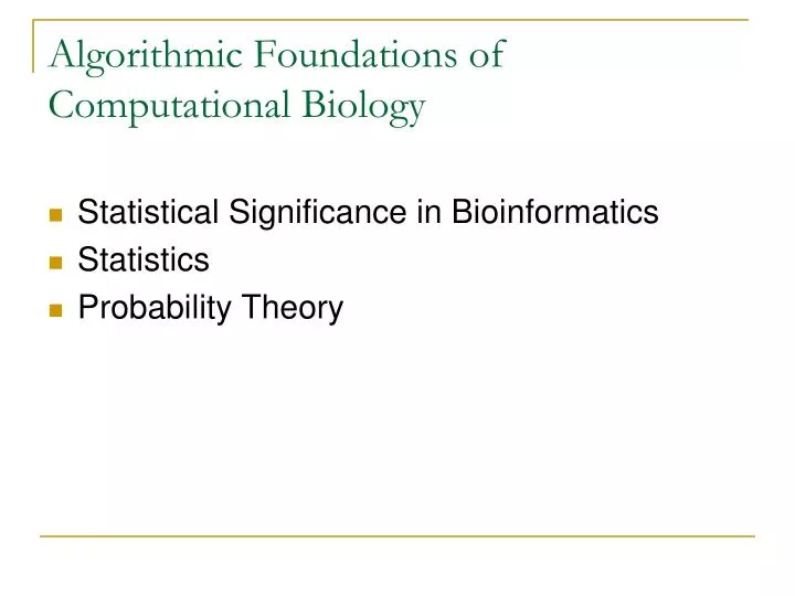
Algorithmic Foundations of Computational Biology . Statistical Significance in Bioinformatics Statistics Probability Theory. SIGNIFICANT SIMILARITY FOR TWO DNA SEQUENCES. AC TACCG CGT A AA TT C TAAC AC ACTTA CGT T AA CC C GGGA. Size of sequences = 20 Number of matches = 8.

E N D
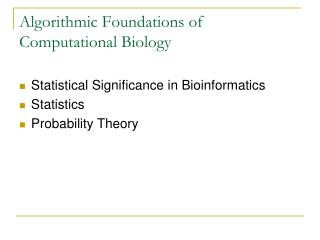
Algorithmic Foundations of Computational Biology • Statistical Significance in Bioinformatics • Statistics • Probability Theory
SIGNIFICANT SIMILARITYFOR TWO DNA SEQUENCES ACTACCGCGTAAATTCTAAC ACACTTACGTTAACCCGGGA Size of sequences = 20 Number of matches = 8 If the sequences were generated at random with 4 letters A, C, G, T, having equal probability of occurrence at any position, then the two sequences should agree at about ¼ of their positions. 20/4=5. But we observe 8 agreements! Is this significant ?
WHAT ARE THE ASSUMPTIONS ? • How unlikely is this outcome if the sequences were generated at random ? • Assumption: Equal probabilities for A, C, G, T at any site • Assumption: Independence of all A, C, G, T involved • Clearly in our case, something other than chance is going on!!!
STATISTICS • Optimal methods for analyzing data generated by a random process • What to measure ? • ACTACCGCGTAAATTCTAAC • ACACTTACGTTAACCCGGGT 8 3
ACCURACY OF ASSUMPTIONS • The probability calculated based on the assumptions about data (equal probability at any site and independence) • Accuracy of conclusions of statistical analysis depends on the accuracy of assumptions made
SIMPLIFYING ASSUMPTIONS • We need to make simplifying assumptions, even when they do not hold. • Required by the complex computations involved
RANDOM VARIABLES • A discrete random variable is a numerical quantity that in some experiment that involves randomness takes one value from some discrete set of values • Rolling a two six-sided dice, the random variable X = “sum of the two outcomes” • Toss of a fair coin, the random variable Y = “number of tosses until the first head appears”
Number of Matches • the number of matches among two random DNA sequences of length 20 is a random variable, denoted Y • The observed value of Y in our example, denoted y, equals 8
PROBABILITY DISTRIBUTION OF A RANDOM VARIABLE • Is the set of values that this random variable can take together with their associated probabilities • Example. Toss a fair coin twice. Let X be the random variable, X = “the number of heads obtained” Values of Y 0 1 2 Probabilities .25 .5 .25
INDEPENDENCE • A central concept in probability and statistics • Two or more events are independent if the outcome of one event does not affect in any way any other event • Discrete random variables are independent if the value of one does not affect in any way the probabilities associated with the possible values of any other random variable
Examples • Different rolls of a die are independent • Different tosses of coin are independent
The BERNOULLI Random Variable • A Bernoulli trial is a single trial with twooutcomes, called“success”and“failure” • The probability of success is denoted p and theprobability of failureisq = 1-p • The Bernoulli random variable is Y= “number of successes” obtained in this trial
The BINOMIAL Distribution • A Binomial random variable is the number of successes in a fixed number of n of independent Bernoulli trials with the same probability of success for each trial • The number of heads in some fixed number of tosses of a coin is an example of a binomial random variable
ASSUMPTIONS “the 4 conditions” • Each trial must result in one of two possible outcomes “success” or “failure” • Trails must be independent • The probability of success must be the same on all trials • The number n of trials must be fixed in advance not determined by the outcomes of the trials
The BINOMIAL Probability Distribution • The Binomial random variable is the variable Y = “number of successes in n trials” = “n choose y”, also known as the Binomial coefficient
Observations • Bernoulli distribution is a special case of the Binomial distribution (when n=1) • p is often an unknown parameter
Careful when using Binomial distribution • Are “the 4 conditions” satisfied ? • When comparing two DNA sequences our question about whether 8 matches are due to chance or not is based on the assumption that the number of matches follow a Binomial distribution • “Success” is the event that two nucleotides in corresponding positions in the two sequences match • ACTACCGCGTAAATTCTAAC • ACACTTACGTTAACCCGGGT
Careful (cont) • It is not necessarily true that the probability of success is the same at all sites • It is not necessarily true that independence holds – population genetics shows that nucleotides frequencies at close sites tend to evolve in dependent fashion leading to dependence of observing a success at very close sites • Thus 2 of “the 4 conditions” for a Binomial distribution do not hold for our pair of DNA sequences comparison
SIMPLIFICATIONS ARE A MUST • Still it might be desirable to make these incorrect assumptions as approximations • Constructing models implies making simplifying assumptions about the process generating the data
The UNIFORM Distribution • The simplest probability distribution • A uniformly distributed random variable Y takes values 1,2,…,m each with same probability
The GEOMETRIC Distribution • Suppose a sequence of independent Bernoulli trials is performed, each having probability of success p • The geometric distributed random variable is the variable Y = “the number of trials before but not including the first failure” • The possible values of the random variable are 1,2,3 ….
The GEOMETRIC Distribution (cont) • The probability of several independent events is the product of their probabilities • For Y= y, there must be y successes followed by one failure • The length of a “successful run” • ACTACCGCGTAAATTCTAAC • ACACTTACGTTAACCCGGGT
The NEGATIVE BINOMIAL Distribution • A sequence of independent Bernoulli trials each with a probability p of success • The Binomial distribution has n such trials with n fixed in advance, and the random variable is the number of successes in these n random trials • In the Generalized Geometric distribution, the number of successes is fixed in advance, at some value m, and the random variable is N the number of trials up to and including this m success • N is said to have the negative binomial distribution
The NEGATIVE BINOMIAL Distribution (cont) • The probability that N=n is the probability that the first n-1 trials result in exactly m-1 successes and n-m failures and the trial n results in success
PROBABILITY THEORY • Probability measures uncertainty • Experiments are performed involving chance or randomness –they are things that can be repeated. • Suppose you roll a pair of dice once. you get a pair of numbers (a,b) such that a = 1,…,6 and b = 1,…,6 • (1,1),(1,2),(1,3),(1,4),(1,5),(1,6), (2,1),(2,2),(2,3),(2,4),(2,5),(2,6), (3,1),(3,2),(3,3),(3,4),(3,5),(3,6), (4,1),(4,2),(4,3),(4,4),(4,5),(4,6), (5,1),(5,2),(5,3),(5,4),(5,5),(5,6), (6,1),(6,2),(6,3),(6,4),(6,5),(6,6) Sample Space Outcomes
PROBABILITY THEORY (cont) • The things that we measure are called events • “Rolling a 7” = {(1,6), (2,5), (3,4), (4,3),(5,2),(6,1)} • We say that the experiment of rolling out a pair of dice give rise to aSample Space S which is just the 36 outcomes possible, and an event is just a set of some of these outcomes.
PROBABILITY THEORY (cont) • Tossing a coin twice • Outcome example: {H,T} • Sample Space S={{H,H}, {H,T},{T,H}, {T,T}} • Event A: “at least one Head occurs” A= {{H,H}, {H,T},{T,H}}
PROBABILITY THEORY (cont) • Sample space provides a mathematical model of real-life situations for which it is supposed to be an abstraction • Mathematical analyses can only be performed on the abstract objects of the sample space and not on real-life situation itself • Since the abstraction resemble the real world you may think that the mathematical relationships you found have something to do with the real world • You can perform now scientific experiments to check out the real world situation
PROBABILITY THEORY (cont) • If you were successful, the mathematical model helped you decipher the real world – you will know this because the results of your experimentsare consistent withthe mathematical relationships your obtained from the model • It could, of course, also happen that your mathematical model was too simple, or otherwise in error and did not give a true picture of the real world. In such a case, the mathematical relationships, while true for the model, cannot be verified by the laboratory experiments. We then need another better model.
PROBABILITY THEORY (cont) • The Sample Space constructed to model a real life situation is a figment of the imagination of the observer of that situation, it depends on what the observers thinks is important. It is not in general unique, and it depends on the subjective interpretation of what is the relevant information.
PROBABILITY THEORY (cont) • Consider the Sample Space S, say with the 36 outcomes of rolling a pair of dice. • To each of the outcome in the sample space associate a number between 0 and 1 such that the sum of these numbers over all outcomes is equal to 1. • The number associated with a particular outcome is called the probability of the outcome, and the entire assignment of probabilities to outcomes is called a probability distribution on S.
PROBABILITY THEORY (cont) • We now define the probability for any event A in the sample space S. • If A is the empty set, P(A)=0. • If then • So given the probability distribution on S we can figure out the probabilities of all events in S.
PROBABILITY SPACE • The sample space with its probability distribution is called a probability space
The Car and Goat Problem • Monty Hall, the master of ceremonies at the “Let’s Make a Deal” game show confronts you wit three closed doors, one of which hides the carof your dreams. Behind each of the other two doors, however, is standing a smelly goat. You will choose a door and win whatever is behind it. • You decide on a door, and announce your choice. • Your host opens then one of the other two doors and reveals a goat. • He then ask you whether you would like to switch your choice to the unopend door that you did not at first choose. • Is it in your advantage to switch ?????? Monty Hall’s game show: “Let’s Make a Deal”
Solution to the Car and Goat Problem • Construct sample space to model the experiment • What is the experiment ? • Want to translate the story into a precise mathematical formulation
Solution to the Car and Goat Problem (cont) • There are three actions: • First you make your initial choice of one of the three possible doors • Monty Hall chooses one of the other doors with a goat behind it • You switch/You do not switch your choice
Solution to the Car and Goat Problem (cont) • Now suppose that the door with the car behind it is labeled 1, and the remaining two doors with goats are labeled 2 and 3. • What is a typical outcome of this game ? • Solution … due next class for extra points
Solution to the Car and Goat Problem (cont) • Example: (1,2,3,L) means “you choose door 1 (with the car behind it), Monty Hall opens door 2, and since you switch, you might switch to 3, thereby losing the car” • The SWITCH sample space is: Sswitch={(1,2,3,L), (1,3,2,L), (2,3,1,W),(3,2,1,W)} We could also use a sample space S’switch={(1,2,3),(1,3,2),(2,3,1),(3,2,1)} Clearly these are the only “plays” possible for our game.
Solution to the Car and Goat Problem (cont) • We want a probability distribution for our sample space. • Real life situation: how do we choose a door ? You probably guess at random. That is, you choose all possibilities equally likely. That is you choose a uniform distribution. Each door has probability 1/3 of being chosen • Event: “Choose door 2” ={(2,3,1,W)} prob 1/3 • Event: “Choose door 3”={(3,2,1,W)} prob 1/3 • Event: “Choose door 1”={(1,2,3,L),(1,3,2,L)} prob 1/3
Solution to the Car and Goat Problem (cont) • Event “You win” ={(2,3,1,W), (3,2,1,W)} • Probability(“You win”)=1/3 + 1/3=2/3 • Event “You lose” ={(1,2,3,L),(1,3,2,L)} • Probability(“You lose”)=1/3
Solution to the Car and Goat Problem (cont) • The NO-SWITCH sample space is: Sno-switch={(1,2,1,W), (1,3,1,W), (2,3,2,L),(3,2,3,L)} Similarly, • Event “You win” ={(1,2,1,W), (1,3,1,W)} • Probability(“You win”)=1/3 • Event “You lose” ={(2,3,2,L),(3,2,3,L)} • Probability(“You lose”)=1/3+1/3=2/3 Conclusion: SWITCH is Better!