Download

1 / 84
1.27k likes | 2.04k Views
Iterative Closest Point. Ronen Gvili www.cs.tau.ac.il/~dcor/Graphics/adv-slides/ ICP .ppt. The Problem. Align two partially- overlapping meshes given initial guess for relative transform. Data Types . Point sets Line segment sets (polylines) Implicit curves : f(x,y,z) = 0

E N D
Iterative Closest Point Ronen Gvili www.cs.tau.ac.il/~dcor/Graphics/adv-slides/ICP.ppt
The Problem • Align two partially-overlapping meshesgiven initial guessfor relative transform
Data Types • Point sets • Line segment sets (polylines) • Implicit curves : f(x,y,z) = 0 • Parametric curves : (x(u),y(u),z(u)) • Triangle sets (meshes) • Implicit surfaces : s(x,y,z) = 0 • Parametric surfaces (x(u,v),y(u,v),z(u,v)))
Motivation • Shape inspection • Motion estimation • Appearance analysis • Texture Mapping • Tracking
Motivation • Range images registration
Motivation • Range images registration
Corresponding Point Set Alignment • Let M be a model point set. • Let S be a scene point set. We assume : • NM = NS. • Each point Si correspond to Mi .
Corresponding Point Set Alignment The MSE objective function : The alignment is :
Aligning 3D Data • If correct correspondences are known, can find correct relative rotation/translation
Aligning 3D Data • How to find correspondences: User input? Feature detection? Signatures? • Alternative: assume closest points correspond
Aligning 3D Data • How to find correspondences: User input? Feature detection? Signatures? • Alternative: assume closest points correspond
Aligning 3D Data • Converges if starting position “close enough“
Closest Point • Given 2 points r1 and r2 , the Euclidean distance is: • Given a point r1 and set of points A , the Euclidean distance is:
Finding Matches • The sceneshape S is aligned to be in the best alignment with the model shape M. • The distance of each point s of the scene from the model is :
Finding Matches C – the closest point operator Y – the set of closest points to S
Finding Matches • Finding each match is performed in O(NM) worst case. • Given Y we can calculate alignment • S is updated to be :
The Algorithm Init the error to ∞ Y = CP(M,S),e Calculate correspondence (rot,trans,d) Calculate alignment S`= rot(S)+trans Apply alignment d` = d Update error If error > threshold
The Algorithm function ICP(Scene,Model) begin E` + ∞; (Rot,Trans) In Initialize-Alignment(Scene,Model); repeat E E`; Aligned-Scene Apply-Alignment(Scene,Rot,Trans); Pairs Return-Closest-Pairs(Aligned-Scene,Model); (Rot,Trans,E`) Update-Alignment(Scene,Model,Pairs,Rot,Trans); Until |E`- E| < Threshold return (Rot,Trans); end
Convergence Theorem • The ICP algorithm always converges monotonically to a local minimum with respect to the MSE distance objective function.
Convergence Theorem • Correspondence error : • Alignment error:
Ek Calculate correspondence Dk Calculate alignment S`= rot(S)+trans Apply alignment Convergence Theorem Ek+1 Calculate correspondence Dk+1 Calculate alignment
Convergence Theorem • Proof :
Convergence Theorem • Proof : If not - the identity transform would yield a smaller MSE than the least square alignment. Apply the alignmentqk on S0 Sk+1 . Assuming the correspondences are maintained: the MSE is still dk.
Convergence Theorem • Proof : After the last alignment, the closest point operator is applied : It is clear that: Thus :
Time analysis Each iteration includes 3 main steps A. Finding the closest points : O(NM) per each point O(NM*NS) total. B. Calculating the alignment: O(NS) C. Updating the scene: O(NS)
Optimizing the Algorithm The best match/nearest neighbor problem : Given N records each described by K real values (attributes) , and a dissimilarity measure D , find the m records closest to a query record.
Optimizing the Algorithm • K-D Tree : Construction time: O(knlogn) Space: O(n) Region Query : O(n1-1/k+k )
Optimizing the Algorithm Optimizing the K-D Tree : • Motivation: In each internal node we can exclude the sub K-D tree if the distance to the partition is greater than the ball radius . • Adjusting the discriminating number, the partition value , and the number of records in each bucket.
Optimizing the Algorithm • Optimizing the K-D Tree : We choose in each internal node the key with the largest spread values as the discriminator and the median as the partition value.
Optimizing the Algorithm • The Optimized K-D Tree : Construction time : Tn = 2Tn/2+kN = O(KNlogN) Search time: O(logN) Expected.
Optimizing the Algorithm • The Optimized K-D Tree : The algorithm can use the m-closest points to cache potentially closest points.
Optimizing the Algorithm • As the ICP algorithm proceeds a sequence of vectors is generated : q1, q2, q3, q4…
Optimizing the Algorithm • Let be a small angular tolerance. • Suppose : • Instead of 50 iterations in the ICP , this accelerated variant converges in less than 20 iterations.
Time analysis Each iteration includes 3 main steps A. Finding the closest points : O(NM) per each point O(NMlogNS) total. B. Calculating the alignment: O(NS) C. Updating the scene: O(NS)
ICP Variants • Variants on the following stages of ICPhave been proposed: • Selecting sample points (from one or both meshes) • Matching to points in the other mesh • Weighting the correspondences • Rejecting certain (outlier) point pairs • Assigning an error metric to the current transform • Minimizing the error metric w.r.t. transformation
Performance of Variants • Can analyze various aspects of performance: • Speed • Stability • Tolerance of noise and/or outliers • Maximum initial misalignment
ICP Variants • Selecting sample points (from one or both meshes). • Matching to points in the other mesh. • Weighting the correspondences. • Rejecting certain (outlier) point pairs. • Assigning an error metric to the current transform. • Minimizing the error metric w.r.t. transformation.
Selection of points • Use all available points [Besl 92]. • Uniform subsampling [Turk 94]. • Random sampling in each iteration [Masuda 96]. • Ensure that samples have normals distributed as uniformly as possible [Rusinkiewicz 01].
Selection of points Uniform Sampling Normal-Space Sampling
ICP Variants • Selecting sample points (from one or both meshes). • Matching to points in the other mesh. • Weighting the correspondences. • Rejecting certain (outlier) point pairs. • Assigning an error metric to the current transform. • Minimizing the error metric w.r.t. transformation.
Points matching • Closest point in the other mesh [Besl 92]. • Normal shooting [Chen 91]. • Reverse calibration [Blais 95]. • Restricting matches to compatible points (color, intensity , normals , curvature ..) [Pulli 99].
Closest point : Points matching
Normal Shooting Points matching