Download

1 / 48
480 likes | 660 Views
Principles of MRI Physics and Engineering. Allen W. Song Brain Imaging and Analysis Center Duke University. Part II.1 Image Formation. What is image formation?. Define the spatial location of the proton pools that contribute to the MR signal. Steps in 3D Localization.

E N D
Principles of MRI Physics and Engineering Allen W. Song Brain Imaging and Analysis Center Duke University
Part II.1 Image Formation
What is image formation? Define the spatial location of the proton pools that contribute to the MR signal.
Steps in 3D Localization • Can only detect total RF signal from inside the “RF coil” (the detecting antenna) • Excite and receive Mxy in a thin (2D) slice of the subject • The RF signal we detect must come from this slice • Reduce dimension from 3D down to 2D • Deliberately make magnetic field strength B depend on location within slice • Frequency of RF signal will depend on where it comes from • Breaking total signal into frequency components will provide more localization information • Make RF signal phase depend on location within slice
RF Field: Excitation Pulse Fo FT Fo Fo+1/ t 0 t Time Frequency Fo Fo FT DF= 1/ t t
Gradient Fields: Spatially Nonuniform B: • Extra static magnetic fields (in addition to B0) that vary their intensity in a linear way across the subject • Precession frequency of M varies across subject • This is called frequency encoding — using a deliberately applied nonuniform field to make the precession frequency depend on location Center frequency [63 MHz at 1.5 T] f 60 KHz Gx = 1 Gauss/cm = 10 mTesla/m = strength of gradient field x-axis Left = –7 cm Right = +7 cm
Exciting and Receiving Mxy in a Thin Slice of Tissue Source of RF frequency on resonance Excite: Addition of small frequency variation Amplitude modulation with “sinc” function RF power amplifier RF coil
Exciting and Receiving Mxy in a Thin Slice of Tissue RF coil Receive: RF preamplifier Filters Analog-to-Digital Converter Computer memory
Determining slice thickness Resonance frequency range as the result of slice-selective gradient: DF = gH * Gsl * dsl The bandwidth of the RF excitation pulse: Dw/2p Thus the slice thickness can be derived as dsl = Dw / (gH * Gsl * 2p)
Changing slice thickness • There are two ways to do this: • Change the slope of the slice selection gradient • Change the bandwidth of the RF excitation pulse • Both are used in practice, with (a) being more popular
Changing slice thickness new slice thickness
Selecting different slices • In theory, there are two ways to select different slices: • Change the position of the zero point of the slice • selection gradient with respect to isocenter • (b) Change the center frequency of the RF to correspond • to a resonance frequency at the desired slice • F = gH (Bo + Gsl * Lsl ) • Option (b) is usually used as it is not easy to change the • isocenter of a given gradient coil.
Selecting different slices new slice location
Readout Localization (frequency encoding) • After RF pulse (B1) ends, acquisition (readout) of NMR RF signal begins • During readout, gradient field perpendicular to slice selection gradient is turned on • Signal is sampled about once every few microseconds, digitized, and stored in a computer • Readout window ranges from 5–100 milliseconds (can’t be longer than about 2T2*, since signal dies away after that) • Computer breaks measured signal V(t) into frequency components v(f) — using the Fourier transform • Since frequency fvaries across subject in a known way, we can assign each component v(f) to the place it comes from
Readout of the MR Signal Constant Magnetic Field Varying Magnetic Field w/o encoding w/ encoding
Readout of the MR Signal Fourier Transform
A typical diagram for MRI frequency encoding: Gradient-echo imaging Excitation Slice Selection TE Frequency Encoding digitizer on Readout
Phase History TE Gradient Phase digitizer on
A typical diagram for MRI frequency encoding: Spin-echo imaging Excitation Slice Selection TE Frequency Encoding digitizer on Readout
Phase History 180o TE Gradient Phase
Image Resolution (in Plane) • Spatial resolution depends on how well we can separate frequencies in the data V(t) • Resolution is proportional to f = frequency accuracy • Stronger gradients nearby positions are better separated in frequencies resolution can be higher for fixed f • Longer readout times can separate nearby frequencies better in V(t) because phases of cos(ft) and cos([f+f]t) will be more different
Calculation of the Field of View (FOV)along frequency encoding direction • * Gf * FOVf = BW, where BW is the bandwidth for the receiver digitizer.
The Second Dimension: Phase Encoding • Slice excitation provides one localization dimension • Frequency encoding provides second dimension • The third dimension is provided by phase encoding: • We make the phase of Mxy (its angle in the xy-plane) signal depend on location in the third direction • This is done by applying a gradient field in the third direction ( to both slice select and frequency encode) • Fourier transform measures phase of each v(f) component ofV(t), as well as the frequency f • By collecting data with many different amounts of phase encoding strength, can break each v(f) into phase components, and so assign them to spatial locations in 3D
A typical diagram for MRI phase encoding:Gradient-echo imaging Excitation Slice Selection Frequency Encoding Phase Encoding digitizer on Readout
A typical diagram for MRI phase encoding: Spin-echo imaging Excitation Slice Selection Frequency Encoding Phase Encoding digitizer on Readout
Calculation of the Field of View (FOV)along phase encoding direction • * Gp * FOVp = Np / Tp where Tp is the duration and Np the number of the phase encoding gradients, Gp is the maximum amplitude of the phase encoding gradient.
Multi-slice acquisition Total acquisition time = Number of views * Number of excitations * TR Is this the best we can do? Interleaved excitation method
Part II.2 Introduction to k-space(a space of the spatial frequency)
Acquired MR Signal Mathematical Representation: This equation is obtained by physically adding all the signals from each voxel up under the gradients we use. From this equation, it can be seen that the acquired MR signal, which is also in a 2-D space (with kx, ky coordinates), is the Fourier Transform of the imaged object.
k-space Image space ky y kx x Acquired Data Final Image Two Spaces IFT FT
The k-space Trajectory Equations that govern k-space trajectory: Kx = g/2p 0tGx(t) dt Ky = g/2p 0tGy(t) dt
A typical diagram for MRI frequency encoding: A k-space perspective Excitation Slice Selection Frequency Encoding digitizer on Readout Exercise drawing its k-space representation
A typical diagram for MRI frequency encoding: A k-space perspective Excitation Slice Selection Frequency Encoding digitizer on Readout Exercise drawing its k-space representation
A typical diagram for MRI phase encoding: A k-space perspective Excitation Slice Selection Frequency Encoding Phase Encoding digitizer on Readout Exercise drawing its k-space representation
A typical diagram for MRI phase encoding: A k-space perspective Excitation Slice Selection Frequency Encoding Phase Encoding digitizer on Readout Exercise drawing its k-space representation
. . . . . . . . . . . . . . . . . . . . . . . . . . . . . . . . . . . . . . . . . . . . . . . . . . . . . . . . . . . . . . . . . . . . . . . . . . . . . . . . . . . . . . . . . . . . . . . . . . . . Sampling in k-space Dk kmax Dk = 1 / FOV 2kmax = 1 / Dx Link back to slides 26 and 30
. . . . . . . . . . . . . . . . . . . . . . . . . . . . . . . . . . . . . . . . . . . . . . . . . . . . . . . . . . . . . . . . . . . . . . . . . . . . . . . . . . . . . . . . . . . . . . . . . . . . . . . . . . . . . . . . . . . . . . . . . . . . . A B FOV: Pixel Size: FOV: 10 cm Pixel Size: 1 cm
. . . . . . . . . . . . . . . . . . . . . . . . . . . . . . . . . . . . . . . . . . . . . . . . . . . . . . . . . . . . . . . . . . . . . . . . . . . . . . . . . . . . . . . . . . . . . . . . . . . . . . . . . . . . . . . . . . . . . . . . . . . . . B A FOV: Pixel Size: FOV: 10 cm Pixel Size: 1 cm
. . . . . . . . . . . . . . . . . . . . . . . . . . . . . . . . . . . . . . . . . . . . . . . . . . . . . . . . . . . . . . . . . . . . . . . . . . . . . . . . . . . . . . . . . . . . . . . . . . . . . . . . . . . . . . . . . . . . . . . . . . . . . . . . . . . . . . . . . . . . . . . . . . . . . . . . . . . . . . . . . . . . . . . . . . . . . . . . . . . . . . . . . . . . . . . . . . . . . . . . A B FOV: Pixel Size: FOV: 10 cm Pixel Size: 1 cm