Download

1 / 63
630 likes | 833 Views
Adaptive Sampling with Topological Scores. Dan Maljovec 1 , Bei Wang 1 , Ana Kupresanin 2 , Gardar Johannesson 2 , Valerio Pascucci 1 , and Peer- Timo Bremer 2 1 SCI Institute, University of Utah 2 Lawrence Livermore National Laboratory. 1. Framework:. 4. 2. 3.

E N D
Adaptive Sampling with Topological Scores Dan Maljovec1, Bei Wang1, Ana Kupresanin2, Gardar Johannesson2, Valerio Pascucci1, and Peer-Timo Bremer2 1SCI Institute, University of Utah 2Lawrence Livermore National Laboratory
1 Framework: 4 2 3
Choosing the “Right” Points 4 Models fit by using 10 training points: True Response Model:
Space-filling Sampling No prior knowledge of the dataset Where should we sample the model?
Space-filling Sampling Fill the domain space as evenly as possible
Space-filling Sampling Obtain responses and fit model
Space-filling Sampling 1 round:
Space-filling Sampling 2 rounds:
Space-filling Sampling 3 rounds:
Space-filling Sampling 4 rounds:
Space-filling Sampling 5 rounds:
Space-filling Sampling Refit after 5 rounds of “filling voids”:
Space-filling Sampling What have we learned? Initial fit Refit after adding 5 points
Topologically-Inspired Adaptive Sampling Starting over
Topologically-Inspired Adaptive Sampling 2 rounds:
Topologically-Inspired Adaptive Sampling 3 rounds:
Topologically-Inspired Adaptive Sampling 4 rounds:
Topologically-Inspired Adaptive Sampling 5 rounds:
Topologically-Inspired Adaptive Sampling Refit after 5 rounds of choosing the most topologically significant point:
Topologically-Inspired Adaptive Sampling What have we learned? Initial fit Refit after adding 5 points
Comparison Initial Fit Space-filling Method Adaptive Method
Comparison True Response Model Space-filling Method Adaptive Method
Measuring Topological Significance These points were selected in topologically significant regions: How do we measure topological impact?
Morse-Smale Complex A partition of the domain into monotonic regions ∩ = Stable Manifolds Unstable Manifolds Morse-Smale Complex
Computing the Morse-Smale Complex Traditionally: • Compute steepest ascent/descent gradient from each point in dataset • Color points twice once by following ascending gradient to maximum & another by descending gradient to minimum • Intersect partitions to form Morse-Smale Complex ∩ = Stable Manifolds Unstable Manifolds Morse-Smale Complex
Computing the Morse-Smale Complex Traditionally: • a. Compute steepest ascent gradient from each point in dataset • a. Color points based on maximum where flow halts
Computing the Morse-Smale Complex Traditionally: • b. Compute steepest descent gradient from each point in dataset • b. Color points based on minimum where flow halts
Computing the Morse-Smale Complex Traditionally: • Intersect partitions to form Morse-Smale Complex ∩ = Stable Manifolds Unstable Manifolds Morse-Smale Complex
Computing the Morse-Smale Complex Traditionally: • Compute steepest ascent/descent gradient from each point in dataset Assumes points have a neighborhood • Color points twice once by following ascending gradient to maximum & another by descending gradient to minimum • Intersect partitions to form Morse-Smale Complex ∩ = Stable Manifolds Unstable Manifolds Morse-Smale Complex
Computing the Approximate Morse-Smale Complex Modified Algorithm: • Compute approximate KNN for a point • Compute steepest ascent/descent gradient from each point’s neighborhood in dataset • Color points by gradient flows • Intersect partitions to form Morse-Smale Complex ∩ = Stable Manifolds Unstable Manifolds Morse-Smale Complex
Tracking Persistence Count the number of connected components belonging to the sub-level sets of the function y c a b d x
Tracking Persistence Every connected component has a birth y c a b d x
Tracking Persistence Every connected component has a birth y c a b d x
Tracking Persistence And every connected component has a death y c a b d x
Tracking Persistence Births and deaths of connected components are tied to critical points of the function y c a b d x
Tracking Persistence Births and deaths of connected components are tied to critical points of the function y c a b d x
Tracking Persistence y c a b d x
Tracking Persistence y death A persistence diagram plots birth-death pairings The function value difference between the critical point pairings is what we define as the persistence of a feature c a b d x birth
Persistence Simplification in 2D In surfaces (and higher dimension corollaries), we have saddle points
Persistence Simplification in 2D We can smooth away noise features by thresholdingcritical point pairs above a certain persistence level
Bottleneck Distance y death Comparing two similar functions persistence diagrams x birth
Bottleneck Distance y death Optimization: minimize the distance between pairs of points in the two plots including the line y=x in both pairs Bottleneck distance – the maximum distance resulting from this pairing x birth
1 Framework: 4 2 3
Selecting Initial Training Data Tests use Latin Hypercube Sampling
Fitting a Statistical Model Experimented with: • Gaussian Process Model • Sparse Online Gaussian Process (C++) • 2 Implementations of MARS with bootstrapping • Earth (CRAN) • MDA (CRAN) • Neural Network with bootstrapping • NNet (CRAN)
Classical Scoring Active-Learning McKay (ALM) • Sample high-frequency or low-confidence regions Delta • Distribute samples in the range space or areas of steep gradient Expected Improvement (EI) • Select points with high uncertainty or large discrepancy with existing data Distance (*DP) • Scaling factor applied to above, creating 3 new scoring functions (ALMDP, DeltaDP, EIDP)
Topological Scoring TOPOP • Average change in persistence of each point computed by comparing the Morse-Smale before and after inserting a candidate TOPOB • Bottleneck distance between persistence diagram of Morse-Smale before and after inserting a candidate point TOPOHP • Highest persistence critical point in Morse-Smale complex constructed from combined training and predicted candidate data
Topological Scoring Average Change in Persistence (TOPOP) • Average change in persistence of each point computed by comparing the Morse-Smale before and after inserting a candidate