Download
1 / 31
310 likes | 431 Views
Tutorial de R e aRT. Pedro Ribeiro de Andrade DSA/CCST/INPE São José dos Campos, 2012. O que é o aRT?. SGBD. Apresentação. http://wiki.dpi.inpe.br/doku.php?id=geopro:pedro:cursoart 4 aulas Aula 1: Introdução ao R Aula 2: Introdução ao Pacote sp Aula 3: Introdução ao aRT

E N D
Tutorial de R e aRT Pedro Ribeiro de Andrade DSA/CCST/INPE São José dos Campos, 2012
O que é o aRT? SGBD
Apresentação • http://wiki.dpi.inpe.br/doku.php?id=geopro:pedro:cursoart • 4 aulas • Aula 1: Introdução ao R • Aula 2: Introdução ao Pacote sp • Aula 3: Introdução ao aRT • Aula 4: aRT avançado
Instalação • Instalar R 2.15.1: www.r-project.org • Instalar o Rstudio: http://rstudio.org/ • Instalar TerraView 4.2.0: www.dpi.inpe.br/terraview • Instalar e configurar MySQL 5.5: www.mysql.com • Baixar e descompactar o arquivo http://www.leg.ufpr.br/~pedro/CDaRT/aula.zip • Executar o Rstudio: • Caso a máquina seja de 64 bits: Tools->Options->R version->change->32 bits. Fechar e abrir o Rstudio novamente. • Tools->Set working directory->Change directory para o diretório da pasta descompactada. • Abrir “gera-bancos.R”, dentro da pasta descompactada. • Alterar a senha para a mesma da instalação do MySQL. • Executar o comando: source("gera-bancos.R"). • Esperar a mensagem: “BANCOS DE DADOS GERADOS COM SUCESSO”
Aula 1:Introdução ao R Pedro Ribeiro de Andrade DSA/CCST/INPE São José dos Campos, 2009 Apresentação baseada no curso “Introdução ao R” (http://www.leg.ufpr.br/Rtutorial/)
Sobre o R • Linguagem e ambiente • Software livre • Similar à linguagem e ambiente S • Multiplataforma ctl <- c(4.17,5.58,5.18,6.11,4.50,4.61,5.17,4.53,5.33,5.14) trt <- c(4.81,4.17,4.41,3.59,5.87,3.83,6.03,4.89,4.32,4.69) group <- gl(2,10,20, labels=c("Ctl","Trt")) weight <- c(ctl, trt) anova(lm.D9 <- lm(weight ~ group)) summary(lm.D90 <- lm(weight ~ group - 1)) opar <- par(mfrow = c(2,2), oma = c(0, 0, 1.1, 0)) plot(lm.D9, las = 1)
Interface gráfica X Linguagem de programação • Curva de aprendizado mais lenta • Flexibilidade • R em específico: métodos refletindo o estado-da-arte • Reprodutibilidade: “the ability of a test or experiment to be accurately reproduced, or replicated, by someone else working independently.”
“Foi um kernel quártico 100x100 com raio 2” k = kernel2d(as.points(bod), bod$poly, h0=2, nx=100, ny=100) plot(bod$poly, asp=1, type="n") image(k, add=TRUE, col=terrain.colors(20)) pointmap(as.points(bod), add=TRUE) polymap(bod$poly, add=TRUE)
Sweave: Reproducible Research Finally we will do a kernel analysis [...] <<>>= raster =kernel2d(as.points(bod), bod$poly, h0=2, nx=100, ny=200) layer.raster <- createLayer(db, l="raster") addRaster(layer.raster, raster) @ To get the layer's geometry call getGeometry [...] <<>>= plot(layer.raster) plot(layer.points,add=TRUE) plot(layer.pol, add=TRUE) @ http://www.leg.ufpr.br/~pedro/aRT/docs/aRTintro.html
Instalação: “R U ready?” • CRAN • Binários: base e contrib • Problemas com Windows Vista (instalar na sua própria pasta)
R como uma calculadora 1+2+3 2+3*4 3/2+1 4*3**3 sqrt(2) sin(3.14159) sin(pi) sqrt(tan(45*pi/180))
Operadores Lógicos 1 == 2 1 != 2 1 <= 2 1 < 2 1 > 2 1 >= 2 T & T T & F T | T T | F ((1 == 2) |(2 > 1)) & (4 >= sqrt(tan(45*pi/180)))
Variáveis x <- sin(pi) x x = sin(pi) sin(pi) -> x y <- sqrt(5) y+x x <- 25 x * sqrt(x) -> x1 x2.1 = sin(x1) x2.2 = cos(x1) xsq = x2.1**2 + x2.2**2
Vetores x <- c(2,3,5,7,11) y <- c(x,13,17,19) xx <- 1:10 xx <- 100:1 seq(1,10,1) seq(1,10,2) seq(10,1,-3) rep(1,10) rep(c(1,2),10) rep(4:1,1:4) rep(c(23, 32, 42), c(3, 1, 2))
Operações com Vetores x <- 1:10 x + 2 sqrt(x) y <- 21:30 x+y y <- c(1,2) x+y length(x) rev(x) summary(x) x**x
Índices de Vetores x[2] y <- x[c(1,3,5)] x[4:7] x[12] x <- c(6,5,6,4,4,3,4,2,3,4) y <- c(5,3,4,2,6,5,4,5,4,3) xeq4 <- x == 4 y[xeq4] x[-3] x[-c(3,4,7)] x[y]
Funções seq(1,27,3) seq(from=1,to=27,by=3) seq(from=1,to=27,length=4) seq(f=1,t=27,l=4) seq(t=27,l=4, f=1) seq(1,4) seq(1) seq() sqrt() ?seq
Matrizes x <- 1:12 xmat <- matrix(x,ncol=3) matrix(x,ncol=3,byrow=T) dim(xmat) summary(xmat) summary(as.numeric(xmat)) x1 <- matrix(1:6,ncol=2) x2 <- matrix(6:1,ncol=3) x1*x2 x1 %*% x2 t(x1)*x2
cbind e rbind COLUMNbind e ROWbind x <- matrix(10:1,ncol=2) y <- cbind(x,1:5) y <- rbind(y,c(99,99,99)) z <- cbind(y,rep(88,6),y) z <- cbind(y,88,y)
Acesso a Matrizes people <- cbind(c(1,2,3,4,5,6),c(43,55,52,23,46,25)) people[1,2] people[1:2,2] people[1,] people[,2] people[-3,] people[people[,2]>50,] people <- people[,c(2,1)]
Matrizes xc = round(runif(10), 2) yc = round(runif(10), 2) xy = cbind(xc, yc) rownames(xy) colnames(xy) rownames(xy)=1:10 xy["2",] # aspas duplas ou simples xy[,"xc"] rownames(xy)=2:11 xy[2:4,] xy[paste(2:4),]
Data frame plot(iris) iris[,3] iris[2,] iris$Sepal.Length iris[1:2, "Sepal.Length"] iris[["Sepal.Width"]] rownames(iris)
Listas person<-list(age=21, name='Fred', score=c(65,78,55)) person$name person$score[2] person[[1]] tt <- t.test(rnorm(1000,mean=1), rnorm(1000,mean=1.2), var.equal=T) is.list(tt) names(tt) tt$p.value tt$estimate
Estruturas de dados • Vetor: coleção unidimensional com valores do mesmo tipo • Matriz: mxn com valores do mesmo tipo • Data Frame: mxn com mesmo tipo em cada coluna • Lista: coleção de vetores de tamanhos distintos
Plotagem x <- 1:20 y <- x**3 plot(x,y) plot(x,y,type="l") # tente também “b”,“o”,“s”,“c”,“h” plot(x,y) points(rev(x),y) lines(x,8000-y, col="blue", lwd=5) plot(x,y) points(rev(x),y,pch=3, col="red") points(x,8000-y,pch="$")
Plotagem plot(1:20, 1:20, pch = 1:20) plot(x,y) lines(x,y,lwd=4) lines(rev(x),y,lty=2) plot(c(0,20),c(-8000,8000),type='n') lines(x,y) lines(x,-y) plot(x,y,xlab="Eixo X aqui",ylab="Eixo Y aqui") title("Título vai aqui!") text(6,4000,"Texto em qualquer lugar")
Plotagem plot(sin, -pi, 2*pi) hist(c(2,2,2,2,2,3,3,3,4,4,5,5)) barplot(table(c(2,2,2,2,2,3,3,3,4,4,5,5))) barplot(table(c(2,2,2,2,2,3,3,3,4,4,5,5)), hor=T) par(mfrow=c(2,2)) plot(x,y) plot(x,log(y)) plot(rev(x),y) plot(rev(x), rev(y)) par(mfrow=c(1,1))
Salvando gráficos jpeg(...) ... dev.off() bmp(...) ... dev.off() png(...) ... dev.off()


![DPGR E/R 49/2006 [Art. 20]](https://cdn2.slideserve.com/4041077/dpgr-e-r-49-2006-art-20-dt.jpg)