Download
1 / 29
290 likes | 461 Views
The Partnership of Pure and Applied Math. David Mumford January, 2013 Sanya City, Hainan, China. Before I begin, I want to show a wheel depicting how I see the relationship of pure and applied math:.

E N D
The Partnership of Pure and Applied Math David Mumford January, 2013 Sanya City, Hainan, China
Before I begin, I want to show a wheel depicting how I see the relationship of pure and applied math: What is applied math? It is the construction and analysis of mathematical models to describe and predict any mathematizableaspect of our world. There can be great synergy between pure and applied math – and but there is also divergence.
Outline • Some Personal History and the contemporary threat to this partnership • Math in Early China was algorithmic and applied, very much like computer code. • ‘Fourier’ Series were invented as an applied tool for astronomy by Clairaut in the mid 18th century. • Combining Markov random fields with Bayes’ Theorem is one of the keys to computer vision • Infinite dimensional differential geometry helps the analysis of medical scans • Words of Caution
1. My own path meandered between pure and applied math • My first venture in math -- a digital computer built in 1952 with my soldering gun and 100 WWII surplus relays. • Then I went on to work at Westinghouse on an analog computer that simulated fast and slow neutron flux in a submarine reactor
Around 1956, listening to the lectures of George Mackey, Lars Ahlfors and Oscar Zariski, I fell in love with abstraction, with the idea of a secret garden containing amazing things that could only be seen with the mind’s eye but never touched: pure math. • Again, in 1982, I read a book by David Marr and realized that animal skills in as basic an area as seeing were immensely subtle and cried out for new mathematical models and was drawn back to applied math. • Finally in 1998, I studied Grenander and Miller’s ideas on warping the medical scan of a patient to a body template and realized that a huge area of the differential geometry of infinite dimensional manifolds was largely unexplored, so got sucked into pure math again – with the help, soon after, of Peter Michor.
But there are dark clouds • I think I understand the very distinctive charms of both pure and applied math, and how tightly they are joined in a symbiotic relationship. • Yet there is a huge tension between them, people rarely cross over or even listen to each other’s lectures. The morning talks all related to physics – yet how many physicist’s talks can you understand? • Pure math believes it is intellectually superior, infinitely deeper; applied math has much more money, support from industry, a sense of belonging to contemporary culture. • This is not healthy. Applied math has always rejuvenated pure, theorems in pure unexpectedly lead to new tools with vast applications.
2. Classical Chinese algebra was algorithmic and applied • The great classic in the Chinese tradition is the “Nine Chapters of the Mathematical Art”, JiǔZhāngSuànShù, 九章算術 • Compiled in the Han Dynasty but based on work from the Warring States or even the Zhou Dynasty, destroyed in the massive book burning of the Qin, the first “cultural revolution”. • Of course, “Pythagoras’s” theorem is in the Nine Chapters (it was also in India c.800 BCE, Babylon c.1800 BCE) but I want to look at algebra.
Rectangular Arrays • This is Chapter 8, 方程 Fang Cheng • Here’s a typical problem (everything is done with problems) • Now sell 2 cows and 5 sheep, to buy 13 pigs. Surplus: 1000 cash. Sell 3 cows and 3 pigs to buy 9 sheep. There is exactly enough cash. Sell 6 sheep and 8 pigs. Then buy 5 cows. There is 600 coins deficit. Tell: what is the price of a cow, a sheep and a pig respectively? • This means the three equations: 2C + 5S −13P = 1000 3C − 9S + 3P = 0 −5C + 6S + 8P = −600 • The solution is found to be C = 1200, S = 500, P = 300.
How it was done • An array of sticks, exactly what we call a matrix, was laid out representing the coefficnts (red if pos, black if neg). • These were manipulated exactly as in Gaussian elimination. • Equations were never used, no symbols for unknowns! • The whole procedure resembles in an uncanny way what goes on in a digital computer today.
The Chinese algorithmic orientation • Nothing like this appears in Europe until 18th cent. Fibonacci’sLiber Abaci (1202) had a confused awkward sort of tabular notation. • Remarkably, in the early Yuan Dynasty, Zhu Shijie (朱世杰) proposed solving n simultaneous polynomial equations in n unknowns, using yet larger arrays for all their coefficients – but still without using x,y, etc. • Their algorithm is very similar to Bayer-Stillman’s computer code ‘Macaulay’. • The same story can be told with Chinese astronomy: code-like algorithms, theory implicit
3. How ‘Fourier’ series were discovered: applied math waiting for pure math to catch up. • Two physical problems which pre-occupied mathematicians in the first half of the 18th century: the motion of a vibrating string with fixed endpts and the perturbations of the moon by the sun. • Both led them (in 1749/1754 resp.) to ‘Fourier’ series (including the formula for its coefficients), but they were distracted by the relationship of a physical variable with a mathematical formula, i.e. not formalizing the concept “function”, so could not make Fourier’s 1822 leap, (also based on an application: heat conduction).
Clairaut, in 1754, studying the three body problem, explicitly asserted that all periodic functions had a trigonometric expansion and gave the inversion formula! So why aren’t these called “Clairaut series”? ………………………………………
Pure math did catch up: here’s how I learned it:(Loomis, Abstract Harmonic Analysis)
But this is how engineers (and I) have taught it: Why, when Gowers won the Fields Medal proving the non-existence of “unconditional bases” in various Banach spaces, did no one explain bases to the general public using the example of musical notes? A spectrogram of a female voice singing do, re, mi, fa, sol, la, ti, do
4. Links of pure and applied math in computer vision – image segmentation • Shah and I introduced a free boundary variational problem for segmenting the domain of a real world image into pieces representing the distinct objects in the scene. Its math (pursued by the French school) is challenging -- still unknown if this is well-posed! Vision-wise, it is a very crude model.
Below left: an example of the simplified Mumford-Shah algorithm on an easy image. Below right: more complex black/white images, human segmentations and one attempt to segment them (in false color).
Gibbs’ random fields and Bayes’ rule:Energy = log(probability) in non-physical settings • These experiments and the work of S. and D. Geman led to a general perspective which underlies much of our present approach to vision.
This link has been very productive. People have gathered probabilities of many aspects of natural images (how likely is an edge caused by a shadow, a crease, foregrnd/backgrnd?) and fed these into Gibbsian models. • But it’s been hard to find algorithms to compute the modes of Gibbs distributions – so engineers rejected this approach for a decade. Now some better algorithms appeared and the approach is popular! • Behind this, there is a big issue of modeling images on a discrete lattice or on R2. I will talk about this in my next lecture.
5. A mathematical model for comparing shapes: use geodesics in a space of submanifolds • Riemann’s Habilitationschiftproposed this idea: “There are however manifolds in which the fixing of position requires not a finite number but either an infinite series or a continuous manifold of determinations of quantity. Such manifolds are constituted for example by … the possible shapes of a figure in space, etc.” • Fixing an ambient manifold M and some topo-logical invariants, let us define the Chow manifolds of M to be the manifolds of all submanifolds of M of the prescribed topological type.
How Riemann’s vision evolved • Arnold made the first step studying a metric on the infinite dimensional manifold of all volume preserving diffeomorphisms of Rn, showing its geodesics were solutions of Euler’s equantion for fluid flow and calculating its curvature. • But it was the application to warping medical images, body parts that has driven the study of a huge variety of other metrics on diffeomorphisms and submanifolds. Marsden and his school picked this up.
A Sobolev-type Riemannian metric and its geodesics – here is an example of Younes Two geodesics:
Now a major industry in analyzing medical scanscomparing the full cortex of a patient with a ‘template’ cortex using sulci, gyri, surface, MRI) • Du, Younes, Qiu, Neuroimage 2011Whole brain diffeomorphic metric mapping • a = healthy brain • d = senile brain with shrunken white matter, enlarged ventricles • c = warp of a, matching d
Kriegl and Michor’s theory of convenient manifolds allows one to use freely Csubmanifolds and do standard differential geometry. One can take Cauchy completions in Sobolev-type Riemannian metrics if preferred. • Strange new beasts occur: e.g. manifolds with local geodesic spray but conjugate points dense and inf(path length)0. • I will discuss some of this theory in my 3rd lecture and apply it to the Yu JiTu禹迹图a Song Dynasty map of China.
6. Words of Caution • Almost all mathematicians, up to 1920 or so, worked on physics and applied as well as pure math • Then Bourbaki on the one hand and the rise of computers on the other pulled them apart. • In 1952 SIAM was founded in the US, followed by ICIAM and all the other “IAM” societies. • Mechanics was dropped as a course in math depts. • CS and Statistics began to form separate departments. Applied math is not one field but the heavy use of computer experiments unites them all. • Physicists dropped all pretense of using rigorous math.
The negative side • Explosion of specialized languages fragmented pure math as well as applied. • How many people can define all of these: • perverse sheaves, • the monster group, • barreled spaces, • inaccessible cardinals • Try explaining a relevant piece of math to a biologist (e.g. who doesn’t know what a group is)! • We have allowed ourselves to live in a tower of Babel. Each field, each sub-sub-field, is going its own way.
There is a culture of modeling as well as its pitfalls Develop pure math theory that is increasingly irrelevant Fall in love with code Tweak endlessly to improve ROC curve
Some words to new students • In my experience, this is a very hard paradigm to teach – students are either by nature more mathy or more engineery and veer off to left or right. • One must not forget that all models are inaccurate simplifications of nature so there will always be errors. Don’t cling to your favorite model! • But all models also have theoretical properties that shed light on what they can and cannot capture and these must not be neglected. Don’t ignore the math. • One must go back and forth between math/experiment. • Thank you for listening.