Download

1 / 107
1.08k likes | 1.33k Views
Text Categorization. Categorization. Problem: Given a universe of objects and a pre-defined set of classes, or categories, assign each object to its correct class. Examples:. Overview. Definition of Text Categorization Techniques Decision Trees Maximum Entropy Modeling

E N D
Categorization • Problem: Given a universe of objects and a pre-defined set of classes, or categories, assign each object to its correct class. • Examples:
Overview • Definition of Text Categorization • Techniques • Decision Trees • Maximum Entropy Modeling • k-Nearest Neighbor Classification
Text categorization • Classification (= Categorization) • Task of assigning objects to classes or categories • Text categorization • Task of classifying the topic or theme of a document
Statistical classification • Training set of objects • Data representation model • Model class • Training procedure • Evaluation
Training set of objects • A set of objects, each labeled by one or more classes • Example from Reuters <REUTERS TOPICS="YES" NEWID="2005"> <DATE> 5-MAR-1987 09:22:57.75</DATE> <TOPICS><D>earn</D></TOPICS> <PLACES><D>usa</D></PLACES> <TEXT> <TITLE>NORD RESOURCES CORP <NRD> 4TH QTR NET</TITLE> <DATELINE> DAYTON, Ohio, March 5 - </DATELINE> <BODY>Shr 19 cts vs 13 cts Net 2,656,000 vs 1,712,000 Revs 15.4 mln vs 9,443,000 Avg shrs 14.1 mln vs 12.6 mln Shr 98 cts vs 77 cts Net 13.8 mln vs 8,928,000 Revs 58.8 mln vs 48.5 mln Avg shrs 14.0 mln vs 11.6 mln NOTE: Shr figures adjusted for 3-for-2 split paid Feb 6, 1987. Reuter </BODY></TEXT> </REUTERS>
Data Representation Model • The training set is encoded via a data representation model • Typically, each object in the training set is represented by a pair (x, c), where: • x: a vector of measurements • c: class label
Data Representation • For text categorization: • use words that are frequent in “earnings” documents • the 20 most representative words are: vs, min, cts, loss, &, 000, profit, dlrs, pct, etc. • Each document is represented as vector where and tfij is the number of occurrences of word i in document j and lj is the length of document j.
Model Class and Training Procedure • Model class • A parameterized family of classifiers • e.g. a model class for binary classification: g(x) = w∙x + w0 • if g(x) > 0, choose class c1, else c2 • Training procedure • Algorithm to select one classifier from this family • i.e., to select proper parameters values (e.g. w, w0)
Evaluation • Borrowing from IR, NLP systems are evaluated by precision, recall, etc. • Example: for text categorization, given a set of documents of which a subset is in a particular category (say, “earnings”), the system classifies some other subset of the documents as belonging to the “earnings” category. • The results of the system are compared with the actual results as follows:
Evaluation measures • Precision • Recall • Accuracy • Error
Evaluation of text categorization • macro-averaging • Compute an evaluation measure for each contingency table separately and average over categories • gives equal weight to each category • macro-averaged precision = • micro-averaging • Make a single contingency table for all categories by summing the scores in each cell, then compute the evaluation measure for the whole table • gives equal weight to each object • micro-averaged precision =
Classification Techniques • Naïve Bayes • Decision Trees • Maximum Entropy Modeling • Support Vector Machines • k-Nearest Neighbor
Bayesian Methods • Learning and classification methods based on probability theory • Bayes theorem plays a critical role in probabilistic learning and classification • Build a generative model that approximates how data is produced • Uses prior probability of each category given no information about an item • Categorization produces a posterior probability distribution over the possible categories given a description of an item
Bayes’ Rule prior probability posterior probability
Maximum likelihood Hypothesis If all hypotheses are a priori equally likely, need only to consider the P(D|h) term:
Naïve Bayes Classifiers Task: Classify a new instance based on a tuple of attribute values
Naïve Bayes Classifier: Assumptions • P(cj) • Can be estimated from the frequency of classes in the training examples. • P(x1,x2,…,xn|cj) • O(|X|n•|C|) • Could only be estimated if a very, very large number of training examples was available. Conditional Independence Assumption: Assume that the probability of observing the conjunction of attributes is equal to the product of the individual probabilities.
Flu X1 X2 X3 X4 X5 runnynose sinus cough fever muscle-ache The Naïve Bayes Classifier • Conditional Independence Assumption: features are independent of each other given the class:
C X1 X2 X3 X4 X5 X6 Learning the Model • Common practice: maximum likelihood • simply use the frequencies in the data
Flu X1 X2 X3 X4 X5 runnynose sinus cough fever muscle-ache Problem with Max Likelihood • What if we have seen no training cases where patient had no flu and muscle aches? • Zero probabilities cannot be conditioned away, no matter the other evidence!
Smoothing to Avoid Overfitting # of values of Xi overall fraction in data where Xi=xi,k • Somewhat more subtle version extent of “smoothing”
Text Classification Using Naïve Bayes:Basic method • Attributes are text positions, values are words. • Naive Bayes assumption is clearly violated. • Example? • Still too many possibilities • Assume that classification is independent of the positions of the words • Use same parameters for each position
Text Classification Algorithms: Learning • From training corpus, extract Vocabulary • Calculate required P(cj)and P(xk | cj)terms • For each cj in Cdo • docsjsubset of documents for which the target class is cj • Textj single document containing all docsj • for each word xkin Vocabulary • nk number of occurrences ofxkin Textj
Text Classification Algorithms: Classifying • positions all word positions in current document which contain tokens found in Vocabulary • Return cNB, where
Naive Bayes Time Complexity • Training Time: O(|D|Ld + |C||V|)) where Ld is the average length of a document in D • Assumes V and all Di , ni, and nij pre-computed in O(|D|Ld) time during one pass through all of the data. • Generally just O(|D|Ld) since usually |C||V| < |D|Ld • Test Time: O(|C| Lt) where Lt is the average length of a test document • Very efficient overall, linearly proportional to the time needed to just read in all the data
Underflow Prevention • Multiplying lots of probabilities, which are between 0 and 1 by definition, can result in floating-point underflow • Since log(xy) = log(x) + log(y), it is better to perform all computations by summing logs of probabilities rather than multiplying probabilities • Class with highest final un-normalized log probability score is still the most probable
Naïve Bayes Posterior Probabilities • Classification results of naïve Bayes (the class with maximum posterior probability) are usually fairly accurate • However, due to the inadequacy of the conditional independence assumption, the actual posterior-probability numerical estimates are not • Output probabilities are generally very close to 0 or 1
Two Models • Model 1: Multivariate binomial • One feature Xw for each word in dictionary • Xw = true in document d if w appears in d • Naive Bayes assumption: • Given the document’s topic, appearance of one word in document tells us nothing about chances that another word appears
Two Models • Model 2: Multinomial • One feature Xi for each word pos in document • feature’s values are all words in dictionary • Value of Xi is the word in position i • Naïve Bayes assumption: • Given the document’s topic, word in one position in document tells us nothing about value of words in other positions • Second assumption: • word appearance does not depend on position for all positions i,j, word w, and class c
Parameter estimation • Binomial model: • Multinomial model: • creating a mega-document for topic j by concatenating all documents in this topic • use frequency of w in mega-document fraction of documents of topic cj in which word w appears fraction of times in which word w appears across all documents of topic cj
Feature selection via Mutual Information • We might not want to use all words, but just reliable, good discriminators • In training set, choose k words which best discriminate the categories. • One way is in terms of Mutual Information: • For each word w and each category c
Feature selection via MI (2) • For each category we build a list of k most discriminating terms. • For example (on 20 Newsgroups): • sci.electronics: circuit, voltage, amp, ground, copy, battery, electronics, cooling, … • rec.autos: car, cars, engine, ford, dealer, mustang, oil, collision, autos, tires, toyota, … • Greedy: does not account for correlations between terms • In general feature selection is necessary for binomial NB, but not for multinomial NB
Evaluating Categorization • Evaluation must be done on test data that are independent of the training data (usually a disjoint set of instances). • Classification accuracy: c/n where n is the total number of test instances and c is the number of test instances correctly classified by the system. • Results can vary based on sampling error due to different training and test sets. • Average results over multiple training and test sets (splits of the overall data) for the best results.
Example: AutoYahoo! • Classify 13,589 Yahoo! webpages in “Science” subtree into 95 different topics (hierarchy depth 2)
Example: WebKB (CMU) • Classify webpages from CS departments into: • student, faculty, course, project
WebKB Experiment • Train on ~5,000 hand-labeled web pages • Cornell, Washington, U.Texas, Wisconsin • Crawl and classify a new site (CMU) • Results:
Importance of Conditional Independence Assume a domain with 20 binary (true/false) attributes A1,…, A20, and two classes c1 and c2. Goal: for any case A=A1,…,A20estimate P(A,ci). A) No independence assumptions: Computation of 221 parameters (one for each combination of values) ! • The training database will not be so large! • Huge Memory requirements / Processing time. • Error Prone (small sample error). B) Strongest conditional independence assumptions (all attributes independent given the class) = Naive Bayes: P(A,ci)=P(A1,ci)P(A2,ci)…P(A20,ci) Computation of 20*22 = 80 parameters. • Space and time efficient. • Robust estimations. • What if the conditional independence assumptions do not hold?? C) More relaxed independence assumptions Tradeoff between A) and B)
Conditions for Optimality of Naïve Bayes Answer Assume two classes c1 and c2. A new case A arrives. NB will classify A to c1if: P(A, c1) > P(A, c2) Fact Sometimes NB performs well even if the Conditional Independence assumptions are badly violated. Questions WHY? And WHEN? Hint Classification is about predicting the correct class label and NOT about accurately estimating probabilities. Despite the big error in estimating the probabilities the classification is still correct. Correct estimation accurate prediction but NOT accurate prediction Correct estimation
Naïve Bayes is Not So Naïve • Naïve Bayes: First and Second place in KDD-CUP 97 competition, among 16 (then) state of the art algorithms Goal: Financial services industry direct mail response prediction model. Predict if the recipient of mail will actually respond to the advertisement – 750,000 records. • Robust to Irrelevant Features Irrelevant Features cancel each other without affecting results Instead Decision Trees & Nearest-Neighbor methods can heavily suffer from this. • Very good in Domains with many equally important features Decision Trees suffer from fragmentation in such cases – especially if little data • A good dependable baseline for text classification (but not the best)! • Optimal if the Independence Assumptions hold: • If assumed independence is correct, then it is the Bayes Optimal Classifier for problem • Very Fast: • Learning with one pass over the data; testing linear in the number of attributes, and document collection size • Low Storage requirements • Handles Missing Values
Interpretability of Naïve Bayes (From R.Kohavi, Silicon Graphics MineSet Evidence Visualizer)
Naïve Bayes Drawbacks • Doesn’t do higher order interactions • Typical example: Chess end games • Each move completely changes the context for the next move • C4.5 99.5 % accuracy : NB 87% accuracy. • What if you have BOTH high order interactions AND few training data? • Doesn’t model features that do not equally contribute to distinguishing the classes. • If few features ONLY mostly determine the class, additional features usually decrease the accuracy. • Because NB gives same weight to all features.
Decision Trees Example: decision whether to assign documents to the category "earning" node 1 7681 articles P(c|n1) = 0.300 split: cts value: 2 cts < 2 cts 2 node 2 5977 articles P(c|n2) = 0.116 split: net value: 1 node 5 1704articles P(c|n5) = 0.943 split: vs value: 2 net < 1 net 1 vs < 2 vs 2 node 3 5436 articles P(c|n3) = 0.050 node 4 541 articles P(c|n4) = 0.649 node 6 201 articles P(c|n6) = 0.694 node 7 1403 articles P(c|n7) = 0.996
Decision Trees - Training procedure (1) • Growing a tree with training data • splitting criterion • for finding the feature and its value on which to split • e.g. maximum information gain • stopping criterion • determines when to stop splitting • e.g. all elements at node have same category • Pruning it back to reasonable size • to avoid overfitting the training set e.g. ‘dlrs’ and ‘pct’ in just one document • to optimize performance