Download
1 / 86
920 likes | 1.32k Views
Computing System Fundamentals/Trends + Review of Performance Evaluation and ISA Design Computing Element Choices: Computing Element Programmability Spatial vs. Temporal Computing Main Processor Types/Applications General Purpose Processor Generations The Von Neumann Computer Model

E N D
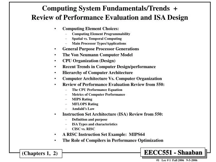
Computing System Fundamentals/Trends + Review of Performance Evaluation and ISA Design • Computing Element Choices: • Computing Element Programmability • Spatial vs. Temporal Computing • Main Processor Types/Applications • General Purpose Processor Generations • The Von Neumann Computer Model • CPU Organization (Design) • Recent Trends in Computer Design/performance • Hierarchy of Computer Architecture • Computer Architecture Vs. Computer Organization • Review of Performance Evaluation Review from 550: • The CPU Performance Equation • Metrics of Computer Performance • MIPS Rating • MFLOPS Rating • Amdahl’s Law • Instruction Set Architecture (ISA) Review from 550: • Definition and purpose • ISA Types and characteristics • CISC vs. RISC • A RISC Instruction Set Example: MIPS64 • The Role of Compilers in Performance Optimization (Chapters 1, 2)
Computing Element Choices • General Purpose Processors (GPPs): Intended for general purpose computing (desktops, servers, clusters..) • Application-Specific Processors (ASPs): Processors with ISAs and architectural features tailored towards specific application domains • E.g Digital Signal Processors (DSPs), Network Processors (NPs), Media Processors, Graphics Processing Units (GPUs), Vector Processors??? ... • Co-Processors: A hardware (hardwired) implementation of specific algorithms with limited programming interface (augment GPPs or ASPs) • Configurable Hardware: • Field Programmable Gate Arrays (FPGAs) • Configurable array of simple processing elements • Application Specific Integrated Circuits (ASICs): A custom VLSI hardware solution for a specific computational task • The choice of one or more depends on a number of factors including: - Type and complexity of computational algorithm (general purpose vs. Specialized) - Desired level of flexibility/ - Performance requirements programmability - Development cost/time - System cost - Power requirements - Real-time constrains The main goal of this course is to study recent architectural design techniques in high-performance GPPs
Computing Element Choices The main goal of this course is the study of recent architectural design techniques in high-performance GPPs General Purpose Processors (GPPs): Flexibility Processor = Programmable computing element that runs programs written using a pre-defined set of instructions Application-Specific Processors (ASPs) Programmability / Configurable Hardware Selection Factors: Co-Processors - Type and complexity of computational algorithms (general purpose vs. Specialized) - Desired level of flexibility - Performance - Development cost - System cost - Power requirements - Real-time constrains Application Specific Integrated Circuits (ASICs) Specialization , Development cost/time Performance/Chip Area/Watt (Computational Efficiency) Performance
Computes one function (e.g. FP-multiply, divider, DCT) Function defined at fabrication time e.g hardware (ASICs) Parameterizable Hardware: Performs limited “set” of functions Computing Element Choices: Computing Element Programmability (Hardware) (Processor) Fixed Function: Programmable: • Computes “any” computable function (e.g. Processors) • Function defined after fabrication • Instruction Set (ISA) e.g. Co-Processors Processor = Programmable computing element that runs programs written using pre-defined instructions
Computing Element Choices: Spatial vs. Temporal Computing Spatial Temporal (using software/program running on a processor) (using hardware) Processor Instructions Processor = Programmable computing element that runs programs written using a pre-defined set of instructions
Main Processor Types/Applications • General Purpose Processors (GPPs) - high performance. • RISC or CISC: Intel P4, IBM Power4, SPARC, PowerPC, MIPS ... • Used for general purpose software • Heavy weight OS - Windows, UNIX • Workstations, Desktops (PC’s), Clusters • Embedded processors and processor cores • e.g: Intel XScale, ARM, 486SX, Hitachi SH7000, NEC V800... • Often require Digital signal processing (DSP) support or other application-specific support (e.g network, media processing) • Single program • Lightweight, often realtime OS or no OS • Examples: Cellular phones, consumer electronics .. (e.g. CD players) • Microcontrollers • Extremely cost/power sensitive • Single program • Small word size - 8 bit common • Highest volume processors by far • Examples: Control systems, Automobiles, toasters, thermostats, ... Increasing Cost/Complexity Increasing volume Examples of Application-Specific Processors
The Processor Design Space Application specific architectures for performance Embedded processors Microprocessors GPPs Real-time constraints Specialized applications Low power/cost constraints Performance is everything & Software rules Performance Microcontrollers The main goal of this course is the study of recent architectural design techniques in high-performance GPPs Cost is everything Chip Area, Power complexity Processor Cost Processor = Programmable computing element that runs programs written using a pre-defined set of instructions
General Purpose Processor Generations Classified according to implementation technology: • The First Generation, 1946-59: Vacuum Tubes, Relays, Mercury Delay Lines: • ENIAC (Electronic Numerical Integrator and Computer): First electronic computer, 18000 vacuum tubes, 1500 relays, 5000 additions/sec (1944). • First stored program computer: EDSAC (Electronic Delay Storage Automatic Calculator), 1949. • The Second Generation, 1959-64: Discrete Transistors. • e.g. IBM Main frames • The Third Generation, 1964-75: Small and Medium-Scale Integrated (MSI) Circuits. • e.g Main frames (IBM 360) , mini computers (DEC PDP-8, PDP-11). • The Fourth Generation, 1975-Present: The Microcomputer. VLSI-based Microprocessors. • First microprocessor: Intel’s 4-bit 4004 (2300 transistors), 1970. • Personal Computer (PCs), laptops, PDAs, servers, clusters … • Reduced Instruction Set Computer (RISC) 1984 (Microprocessor = VLSI-based Single-chip processor) Common factor among all generations: All target the The Von Neumann Computer Model or paradigm
- Control Input Memory (instructions, data) Datapath registers ALU, buses Output CPU Computer System I/O Devices The Von Neumann Computer Model • Partitioning of the programmable computing engine into components: • Central Processing Unit (CPU): Control Unit (instruction decode , sequencing of operations), Datapath (registers, arithmetic and logic unit, buses). • Memory: Instruction and operand storage. • Input/Output (I/O) sub-system: I/O bus, interfaces, devices. • The stored program concept: Instructions from an instruction set are fetched from a common memory and executed one at a time AKA Program Counter PC-Based Architecture The Program Counter (PC) points to next instruction to be processed Major CPU Performance Limitation: The Von Neumann computing model implies sequential execution one instruction at a time Another Performance Limitation: Separation of CPU and memory (The Von Neumann memory bottleneck)
Instruction Fetch Instruction Decode Operand Fetch Execute Result Store Next Instruction Generic CPU Machine Instruction Processing Steps (Implied by The Von Neumann Computer Model) Obtain instruction from program storage The Program Counter (PC) points to next instruction to be processed Determine required actions and instruction size Locate and obtain operand data Compute result value or status Deposit results in storage for later use Determine successor or next instruction (i.e Update PC) Major CPU Performance Limitation: The Von Neumann computing model implies sequential execution one instruction at a time
CPU Organization (Design) Components & their connections needed by ISA instructions • Datapath Design: • Capabilities & performance characteristics of principal Functional Units (FUs): • (e.g., Registers, ALU, Shifters, Logic Units, ...) • Ways in which these components are interconnected (buses connections, multiplexors, etc.). • How information flows between components. • Control Unit Design: • Logic and means by which such information flow is controlled. • Control and coordination of FUs operation to realize the targeted Instruction Set Architecture to be implemented (can either be implemented using a finite state machine or a microprogram). • Description of hardware operations with a suitable language, possibly using Register Transfer Notation (RTN). Control/sequencing of operations of datapath components to realize ISA instructions (From 550)
Recent Trends in Computer Design • The cost/performance ratio of computing systems have seen a steady decline due to advances in: • Integrated circuit technology: decreasing feature size, • Clock rate improves roughly proportional to improvement in • Number of transistors improves proportional to (or faster). • Architectural improvements in CPU design. • Microprocessor systems directly reflect IC and architectural improvement in terms of a yearly 35 to 55% improvement in performance. • Assembly language has been mostly eliminated and replaced by other alternatives such as C or C++ • Standard operating Systems (UNIX, Windows) lowered the cost of introducing new architectures. • Emergence of RISC architectures and RISC-core (x86) architectures. • Adoption of quantitative approaches to computer design based on empirical performance observations. • Increased importance of exploiting thread-level parallelism (TLP) in main-stream computing systems. e.g Multiple processor cores on a single chip
1000 Supercomputers 100 Mainframes 10 Minicomputers Microprocessors 1 0.1 1965 1970 1975 1980 1985 1990 1995 2000 Year Processor Performance Trends Mass-produced microprocessors a cost-effective high-performance replacement for custom-designed mainframe/minicomputer CPUs
Microprocessor Performance 1987-97 Integer SPEC92 Performance > 100x performance increase in the last decade
10,000 100 Intel Processor freq IBM Power PC scales by 2X per DEC generation Gate delays/clock 21264S 1,000 21164A 21264 Pentium(R) 21064A Gate Delays/ Clock Mhz 10 21164 II 21066 MPC750 604 604+ Pentium Pro 100 (R) 601, 603 Pentium(R) 486 386 10 1 1987 1989 1991 1993 1995 1997 1999 2001 2003 2005 Microprocessor Frequency Trend Realty Check: Clock frequency scaling is slowing down! (Did silicone finally hit the wall?) Why? 1- Power leakage 2- Clock distribution delays Result: Deeper Pipelines Longer stalls Higher CPI (lowers effective performance per cycle) ? Frequency doubles each generation Number of gates/clock reduce by 25% Leads to deeper pipelines with more stages (e.g Intel Pentium 4E has 30+ pipeline stages) T = I x CPI x C
Alpha 21264: 15 million Pentium Pro: 5.5 million PowerPC 620: 6.9 million Alpha 21164: 9.3 million Sparc Ultra: 5.2 million Moore’s Law Moore’s Law: 2X transistors/Chip Every 1.5 years (circa 1970) Microprocessor Transistor Count Growth Rate Currently > 1 Billion Still holds today ~ 500,000x transistor density increase in the last 35 years
Computer Technology Trends:Evolutionary but Rapid Change • Processor: • 1.5-1.6 performance improvement every year; Over 100X performance in last decade. • Memory: • DRAM capacity: > 2x every 1.5 years; 1000X size in last decade. • Cost per bit: Improves about 25% or more per year. • Only 15-25% performance improvement per year. • Disk: • Capacity: > 2X in size every 1.5 years. • Cost per bit: Improves about 60% per year. • 200X size in last decade. • Only 10% performance improvement per year, due to mechanical limitations. • Expected State-of-the-art PC by end of year 2006 : • Processor clock speed: ~ 3000 MegaHertz (3 Giga Hertz) • Memory capacity: > 4000 MegaByte (4 Giga Bytes) • Disk capacity: > 500 GigaBytes (0.5 Tera Bytes) Performance gap compared to CPU performance causes system performance bottlenecks With 2-4 processor cores on a single chip
Application Operating System Compiler Firmware Instruction Set Architecture Instr. Set Proc. I/O system Datapath & Control Digital Design Circuit Design Layout Hierarchy of Computer Architecture High-Level Language Programs Assembly Language Programs Software Machine Language Program e.g. BIOS (Basic Input/Output System) e.g. BIOS (Basic Input/Output System) Software/Hardware Boundary (ISA) The ISA forms an abstraction layer that sets the requirements for both complier and CPU designers Microprogram Hardware Register Transfer Notation (RTN) Logic Diagrams VLSI placement & routing Circuit Diagrams
Computer Architecture Vs. Computer Organization • The term Computer architecture is sometimes erroneously restricted to computer instruction set design, with other aspects of computer design called implementation • More accurate definitions: • Instruction set architecture (ISA): The actual programmer-visible instruction set and serves as the boundary between the software and hardware. • Implementation of a machine has two components: • Organization: includes the high-level aspects of a computer’s design such as: The memory system, the bus structure, the internal CPU unit which includes implementations of arithmetic, logic, branching, and data transfer operations. • Hardware: Refers to the specifics of the machine such as detailed logic design and packaging technology. • In general, Computer Architecture refers to the above three aspects: Instruction set architecture, organization, and hardware. The ISA forms an abstraction layer that sets the requirements for both complier and CPU designers CPU Micro- architecture (CPU design) Hardware design and implementation
The Task of A Computer Designer • Determine what attributes that are important to the design of the new machine (CPU). • Design a machine to maximize performance while staying within cost and other constraints and metrics. • It involves more than instruction set design. • Instruction set architecture. • CPU Micro-architecture (CPU design). • Implementation. • Implementation of a machine has two components: • Organization. • Hardware. e.g Power consumption Heat dissipation Real-time constraints (ISA)
Recent Architectural Improvements • Long memory latency-hiding techniques, including: • Increased optimization and utilization of cache systems. • Improved handling of pipeline hazards. • Improved hardware branch prediction techniques. • Optimization of pipelined instruction execution: • Dynamic hardware-based pipeline scheduling. • Dynamic speculative execution. • Exploiting Instruction-Level Parallelism (ILP) in terms of multiple-instruction issue and multiple hardware functional units. • Inclusion of special instructions to handle multimedia applications (limited vector processing). • High-speed bus designs to improve data transfer rates. - Also, increased utilization of point-to-point interconnects instead of one system bus (e.g HyperTransport)
Memory Controller NICs Memory Computer System Components CPU Core 1 GHz - 3.8 GHz 4-way Superscaler RISC or RISC-core (x86): Deep Instruction Pipelines Dynamic scheduling Multiple FP, integer FUs Dynamic branch prediction Hardware speculation Recently 1 or 2 processor cores per chip All Non-blocking caches L1 16-128K 1-2 way set associative (on chip), separate or unified L2 256K- 2M 4-32 way set associative (on chip) unified L3 2-16M 8-32 way set associative (off or on chip) unified L1 L2 L3 CPU Examples: Alpha, AMD K7: EV6, 200-400 MHz Intel PII, PIII: GTL+ 133 MHz Intel P4 800 MHz Caches SDRAM PC100/PC133 100-133MHZ 64-128 bits wide 2-way inteleaved ~ 900 MBYTES/SEC )64bit) Double Date Rate (DDR) SDRAM PC3200 200 MHZ DDR 64-128 bits wide 4-way interleaved ~3.2 GBYTES/SEC (one 64bit channel) ~6.4 GBYTES/SEC (two 64bit channels) RAMbus DRAM (RDRAM) 400MHZ DDR 16 bits wide (32 banks) ~ 1.6 GBYTES/SEC Front Side Bus (FSB) Off or On-chip adapters I/O Buses Current Standard Example: PCI, 33-66MHz 32-64 bits wide 133-528 MBYTES/SEC PCI-X 133MHz 64 bit 1024 MBYTES/SEC Memory Bus Controllers Disks Displays Keyboards Networks I/O Devices: I/O Subsystem North Bridge South Bridge Chipset
Clock cycle cycle 1 cycle 2 cycle 3 CPU Performance Evaluation:Cycles Per Instruction (CPI) • Most computers run synchronously utilizing a CPU clock running at a constant clock rate: where: Clock rate = 1 / clock cycle • The CPU clock rate depends on the specific CPU organization (design) and hardware implementation technology (VLSI) used • A computer machine (ISA) instruction is comprised of a number of elementary or micro operations which vary in number and complexity depending on the instruction and the exact CPU organization (Design) • A micro operation is an elementary hardware operation that can be performed during one CPU clock cycle. • This corresponds to one micro-instruction in microprogrammed CPUs. • Examples: register operations: shift, load, clear, increment, ALU operations: add , subtract, etc. • Thus a single machine instruction may take one or more CPU cycles to complete termed as the Cycles Per Instruction (CPI). • Average CPI of a program: The average CPI of all instructions executed in the program on a given CPU design. (From 550) Instructions Per Cycle = IPC = 1/CPI
Computer Performance Measures: Program Execution Time • For a specific program compiled to run on a specific machine (CPU) “A”, the following parameters are provided: • The total instruction count of the program. • The average number of cycles per instruction (average CPI). • Clock cycle of machine “A” • How can one measure the performance of this machine running this program? • Intuitively the machine is said to be faster or has better performance running this program if the total execution time is shorter. • Thus the inverse of the total measured program execution time is a possible performance measure or metric: PerformanceA = 1 / Execution TimeA How to compare performance of different machines? What factors affect performance? How to improve performance? I CPI C (From 550)
PerformanceA Execution TimeB Speedup = n = = PerformanceB Execution TimeA Comparing Computer Performance Using Execution Time • To compare the performance of two machines (or CPUs) “A”, “B” running a given specific program: PerformanceA = 1 / Execution TimeA PerformanceB = 1 / Execution TimeB • Machine A is n times faster than machine B means (or slower? if n < 1) : • Example: For a given program: Execution time on machine A: ExecutionA = 1 second Execution time on machine B: ExecutionB = 10 seconds PerformanceA / = Execution TimeB / Execution TimeA PerformanceB = 10 / 1 = 10 The performance of machine A is 10 times the performance of machine B when running this program, or: Machine A is said to be 10 times faster than machine B when running this program. (i.e Speedup is ratio of performance, no units) Speedup= The two CPUs may target different ISAs provided the program is written in a high level language (HLL) (From 550)
CPU time = Seconds = Instructions x Cycles x Seconds Program Program Instruction Cycle CPU Execution Time: The CPU Equation • A program is comprised of a number of instructions executed , I • Measured in: instructions/program • The average instruction executed takes a number of cycles per instruction (CPI) to be completed. • Measured in: cycles/instruction, CPI • CPU has a fixed clock cycle time C = 1/clock rate • Measured in: seconds/cycle • CPU execution time is the product of the above three parameters as follows: Or Instructions Per Cycle (IPC): IPC= 1/CPI Executed T = I x CPI x C execution Time per program in seconds Number of instructions executed Average CPI for program CPU Clock Cycle (This equation is commonly known as the CPU performance equation) (From 550)
CPU time = Seconds = Instructions x Cycles x Seconds Program Program Instruction Cycle CPU Execution Time: Example • A Program is running on a specific machine with the following parameters: • Total executed instruction count: 10,000,000 instructions Average CPI for the program: 2.5 cycles/instruction. • CPU clock rate: 200 MHz. (clock cycle = 5x10⁻⁹ seconds) • What is the execution time for this program: CPU time = Instruction count x CPIx Clock cycle = 10,000,000 x 2.5 x 1 / clock rate = 10,000,000 x 2.5 x 5x10-9 = .125 seconds T = I x CPI x C (From 550)
CPU Time = Instruction count x CPIx Clock cycle Depends on: Program Used Compiler ISA Instruction Count I Depends on: Program Used Compiler ISA CPU Organization Depends on: CPU Organization Technology (VLSI) CPI Clock Cycle C Aspects of CPU Execution Time T = I x CPI x C (executed) (Average CPI) (From 550)
CPU time = Seconds = Instructions x Cycles x Seconds Program Program Instruction Cycle Factors Affecting CPU Performance Instruction Count I CPI Clock Cycle C Program X X X Compiler X Instruction Set Architecture (ISA) X X X X Organization (CPU Design) Technology (VLSI) X T = I x CPI x C (From 550)
Speedup = Old Execution Time = Iold x CPIold x Clock cycleold New Execution Time Inew x CPInew x Clock Cyclenew Performance Comparison: Example • From the previous example: A Program is running on a specific machine with the following parameters: • Total executed instruction count, I: 10,000,000 instructions • Average CPI for the program: 2.5 cycles/instruction. • CPU clock rate: 200 MHz. • Using the same program with these changes: • A new compiler used: New instruction count 9,500,000 New CPI: 3.0 • Faster CPU implementation: New clock rate = 300 MHZ • What is the speedup with the changes? Speedup = (10,000,000 x 2.5 x 5x10-9) / (9,500,000 x 3 x 3.33x10-9 ) = .125 / .095 = 1.32 or 32 % faster after changes. Clock Cycle = 1/ Clock Rate (From 550)
Instruction Types & CPI • Given a program with n types or classes of instructions executed on a given CPU with the following characteristics: Ci = Count of instructions of typei CPIi = Cycles per instruction for typei Then: CPI = CPU Clock Cycles / Instruction Count I Where: Instruction Count I = S Ci Executed i = 1, 2, …. n Executed Executed T = I x CPI x C (From 550)
Instruction class CPI A 1 B 2 C 3 Instruction counts for instruction class Code Sequence A B C 1 2 1 2 2 4 1 1 Instruction Types & CPI: An Example • An instruction set has three instruction classes: • Two code sequences have the following instruction counts: • CPU cycles for sequence 1 = 2 x 1 + 1 x 2 + 2 x 3 = 10 cycles CPI for sequence 1 = clock cycles / instruction count = 10 /5 = 2 • CPU cycles for sequence 2 = 4 x 1 + 1 x 2 + 1 x 3 = 9 cycles CPI for sequence 2 = 9 / 6 = 1.5 For a specific CPU design CPI = CPU Cycles / I (From 550)
CPIi x Fi CPI Instruction Frequency & CPI • Given a program with n types or classes of instructions with the following characteristics: Ci = Count of instructions of typei CPIi = Average cycles per instruction of typei Fi = Frequency or fraction of instruction typei executed = Ci/ total executed instruction count = Ci/ I Then: i = 1, 2, …. n Fraction of total execution time for instructions of type i = (From 550)
CPIi x Fi Base Machine (Reg / Reg) Op Freq, Fi CPIi CPIi x Fi % Time ALU 50% 1 .5 23% = .5/2.2 Load 20% 5 1.0 45% = 1/2.2 Store 10% 3 .3 14% = .3/2.2 Branch 20% 2 .4 18% = .4/2.2 CPI Typical Mix Instruction Type Frequency & CPI: A RISC Example Program Profile or Executed Instructions Mix Given Sum = 2.2 CPI = .5 x 1 + .2 x 5 + .1 x 3 + .2 x 2 = 2.2 = .5 + 1 + .3 + .4 (From 550)
Metrics of Computer Performance (Measures) Execution time: Target workload, SPEC, etc. Application Programming Language Compiler (millions) of Instructions per second – MIPS (millions) of (F.P.) operations per second – MFLOP/s ISA Datapath Megabytes per second. Control Function Units Cycles per second (clock rate). Transistors Wires Pins Each metric has a purpose, and each can be misused.
Choosing Programs To Evaluate Performance Levels of programs or benchmarks that could be used to evaluate performance: • Actual Target Workload: Full applications that run on the target machine. • Real Full Program-based Benchmarks: • Select a specific mix or suite of programs that are typical of targeted applications or workload (e.g SPEC95, SPEC CPU2000). • Small “Kernel” Benchmarks: • Key computationally-intensive pieces extracted from real programs. • Examples: Matrix factorization, FFT, tree search, etc. • Best used to test specific aspects of the machine. • Microbenchmarks: • Small, specially written programs to isolate a specific aspect of performance characteristics: Processing: integer, floating point, local memory, input/output, etc.
Types of Benchmarks Cons Pros • Very specific. • Non-portable. • Complex: Difficult • to run, or measure. • Representative Actual Target Workload • Portable. • Widely used. • Measurements • useful in reality. • Less representative • than actual workload. Full Application Benchmarks • Easy to “fool” by designing hardware to run them well. Small “Kernel” Benchmarks • Easy to run, early in the design cycle. • Peak performance results may be a long way from real application performance • Identify peak performance and potential bottlenecks. Microbenchmarks
SPEC: System Performance Evaluation Cooperative The most popular and industry-standard set of CPU benchmarks. • SPECmarks, 1989: • 10 programs yielding a single number (“SPECmarks”). • SPEC92, 1992: • SPECInt92 (6 integer programs) and SPECfp92 (14 floating point programs). • SPEC95, 1995: • SPECint95 (8 integer programs): • go, m88ksim, gcc, compress, li, ijpeg, perl, vortex • SPECfp95 (10 floating-point intensive programs): • tomcatv, swim, su2cor, hydro2d, mgrid, applu, turb3d, apsi, fppp, wave5 • Performance relative to a Sun SuperSpark I (50 MHz) which is given a score of SPECint95 = SPECfp95 = 1 • SPEC CPU2000, 1999: • CINT2000 (11 integer programs). CFP2000 (14 floating-point intensive programs) • Performance relative to a Sun Ultra5_10 (300 MHz) which is given a score of SPECint2000 = SPECfp2000 = 100 All based on execution time and give speedup over a reference CPU
SPEC CPU2000 Programs Benchmark Language Descriptions 164.gzip C Compression 175.vpr C FPGA Circuit Placement and Routing 176.gcc C C Programming Language Compiler 181.mcf C Combinatorial Optimization 186.crafty C Game Playing: Chess 197.parser C Word Processing 252.eon C++ Computer Visualization 253.perlbmk C PERL Programming Language 254.gap C Group Theory, Interpreter 255.vortex C Object-oriented Database 256.bzip2 C Compression 300.twolf C Place and Route Simulator 168.wupwise Fortran 77 Physics / Quantum Chromodynamics 171.swim Fortran 77 Shallow Water Modeling 172.mgrid Fortran 77 Multi-grid Solver: 3D Potential Field 173.applu Fortran 77 Parabolic / Elliptic Partial Differential Equations 177.mesa C 3-D Graphics Library 178.galgel Fortran 90 Computational Fluid Dynamics 179.art C Image Recognition / Neural Networks 183.equake C Seismic Wave Propagation Simulation 187.facerec Fortran 90 Image Processing: Face Recognition 188.ammp C Computational Chemistry 189.lucas Fortran 90 Number Theory / Primality Testing 191.fma3d Fortran 90 Finite-element Crash Simulation 200.sixtrack Fortran 77 High Energy Nuclear Physics Accelerator Design 301.apsi Fortran 77 Meteorology: Pollutant Distribution CINT2000 (Integer) CFP2000 (Floating Point) Programs application domain: Engineering and scientific computation Source: http://www.spec.org/osg/cpu2000/
Top 20 SPEC CPU2000 Results (As of March 2002) Top 20 SPECint2000 Top 20 SPECfp2000 # MHz Processor int peak int base MHz Processor fp peak fp base 1 1300 POWER4 814 790 1300 POWER4 1169 1098 2 2200 Pentium 4 811 790 1000 Alpha 21264C 960 776 3 2200 Pentium 4 Xeon 810 788 1050 UltraSPARC-III Cu 827 701 4 1667 Athlon XP 724 697 2200 Pentium 4 Xeon 802 779 5 1000 Alpha 21264C 679 621 2200 Pentium 4 801 779 6 1400 Pentium III 664 648 833 Alpha 21264B 784 643 7 1050 UltraSPARC-III Cu 610 537 800 Itanium 701 701 8 1533 Athlon MP 609 587 833 Alpha 21264A 644 571 9 750 PA-RISC 8700 604 568 1667 Athlon XP 642 596 10 833 Alpha 21264B 571 497 750 PA-RISC 8700 581 526 11 1400 Athlon 554 495 1533 Athlon MP 547 504 12 833 Alpha 21264A 533 511 600 MIPS R14000 529 499 13 600 MIPS R14000 500 483 675 SPARC64 GP 509 371 14 675 SPARC64 GP 478 449 900 UltraSPARC-III 482 427 15 900 UltraSPARC-III 467 438 1400 Athlon 458 426 16 552 PA-RISC 8600 441 417 1400 Pentium III 456 437 17 750 POWER RS64-IV 439 409 500 PA-RISC 8600 440 397 18 700 Pentium III Xeon 438 431 450 POWER3-II 433 426 19 800 Itanium 365 358 500 Alpha 21264 422 383 20 400 MIPS R12000 353 328 400 MIPS R12000 407 382 Source: http://www.aceshardware.com/SPECmine/top.jsp
Computer Performance Measures : MIPS (Million Instructions Per Second) Rating • For a specific program running on a specific CPU the MIPS rating is a measure of how many millions of instructions are executed per second: MIPS Rating = Instruction count / (Execution Time x 106) = Instruction count / (CPU clocks x Cycle time x 106) = (Instruction count x Clock rate) / (Instruction count x CPI x 106) = Clock rate / (CPI x 106) • Major problem with MIPS rating: As shown above the MIPS rating does not account for the count of instructions executed (I). • A higher MIPS rating in many cases may not mean higher performance or better execution time. i.e. due to compiler design variations. • In addition the MIPS rating: • Does not account for the instruction set architecture (ISA) used. • Thus it cannot be used to compare computers/CPUs with different instruction sets. • Easy to abuse: Program used to get the MIPS rating is often omitted. • Often the Peak MIPS rating is provided for a given CPU which is obtained using a program comprised entirely of instructions with the lowest CPI for the given CPU design which does not represent real programs. (From 550)
Computer Performance Measures : MIPS (Million Instructions Per Second) Rating • Under what conditions can the MIPS rating be used to compare performance of different CPUs? • The MIPS rating is only valid to compare the performance of different CPUs provided that the following conditions are satisfied: • The same program is used (actually this applies to all performance metrics) • The same ISA is used • The same compiler is used • (Thus the resulting programs used to run on the CPUs and obtain the MIPS rating are identical at the machine code level including the same instruction count) (binary) (From 550)
Instruction class CPI A 1 B 2 C 3 Instruction counts (in millions) for each instruction class Code from: A B C Compiler 1 5 1 1 Compiler 2 10 1 1 Compiler Variations, MIPS, Performance: An Example • For the machine with instruction classes: • For a given program two compilers produced the following instruction counts: • The machine is assumed to run at a clock rate of 100 MHz (From 550)
Compiler Variations, MIPS, Performance: An Example (Continued) MIPS = Clock rate / (CPI x 106) = 100 MHz / (CPI x 106) CPI = CPU execution cycles / Instructions count CPU time = Instruction count x CPI / Clock rate • For compiler 1: • CPI1 = (5 x 1 + 1 x 2 + 1 x 3) / (5 + 1 + 1) = 10 / 7 = 1.43 • MIP Rating1 = 100 / (1.428 x 10⁶) = 70.0 • CPU time1 = ((5 + 1 + 1) x 106 x 1.43) / (100 x 106) = 0.10 seconds • For compiler 2: • CPI2 = (10 x 1 + 1 x 2 + 1 x 3) / (10 + 1 + 1) = 15 / 12 = 1.25 • MIPS Rating2= 100 / (1.25 x 10⁶) = 80.0 • CPU time2 = ((10 + 1 + 1) x 106 x 1.25) / (100 x 106) = 0.15 seconds MIPS rating indicates that compiler 2 is better while in reality the code produced by compiler 1 is faster
High Memory $6 points here X[999] Last element to compute X[998] . . . . $2 initially points here First element to compute X[0] Low Memory MIPS32(The ISA not the metric)Loop Performance Example For the loop: for (i=0; i<1000; i=i+1){ x[i] = x[i] + s; } MIPS32 assembly code is given by: lw $3, 8($1) ; load s in $3 addi $6, $2, 4000 ; $6 = address of last element + 4 loop: lw $4, 0($2) ; load x[i] in $4 add $5, $4, $3 ; $5 has x[i] + s sw $5, 0($2) ; store computed x[i] addi $2, $2, 4 ; increment $2 to point to next x[ ] element bne $6, $2, loop ; last loop iteration reached? The MIPS code is executed on a specific CPU that runs at 500 MHz (clock cycle = 2ns = 2x10⁻⁹ seconds) with following instruction type CPIs : For this MIPS code running on this CPU find: 1- Fraction of total instructions executed for each instruction type 2- Total number of CPU cycles 3- Average CPI 4- Fraction of total execution time for each instructions type 5- Execution time 6- MIPS rating , peak MIPS rating for this CPU Instruction type CPI ALU 4 Load 5 Store 7 Branch 3 X[ ] array of words in memory, base address in $2 , s a constant word value in memory, address in $1 From 550
MIPS32 (The ISA) Loop Performance Example (continued) • The code has 2 instructions before the loop and 5 instructions in the body of the loop which iterates 1000 times, • Thus: Total instructions executed, I = 5x1000 + 2 = 5002 instructions • Number of instructions executed/fraction Fi for each instruction type: • ALU instructions = 1 + 2x1000 = 2001 CPIALU = 4 FractionALU = FALU = 2001/5002 = 0.4 = 40% • Load instructions = 1 + 1x1000 = 1001 CPILoad = 5 FractionLoad = FLoad = 1001/5002= 0.2 = 20% • Store instructions = 1000 CPIStore = 7 FractionStore = FStore = 1000/5002 = 0.2 = 20% • Branch instructions = 1000 CPIBranch = 3 FractionBranch= FBranch = 1000/5002= 0.2 = 20% = 2001x4 + 1001x5 + 1000x7 + 1000x3 = 23009 cycles • Average CPI = CPU clock cycles / I = 23009/5002 = 4.6 • Fraction of execution time for each instruction type: • Fraction of time for ALU instructions = CPIALU x FALU / CPI= 4x0.4/4.6 = 0.348 = 34.8% • Fraction of time for load instructions = CPIload x Fload / CPI= 5x0.2/4.6 = 0.217 = 21.7% • Fraction of time for store instructions = CPIstore x Fstore / CPI= 7x0.2/4.6 = 0.304 = 30.4% • Fraction of time for branch instructions = CPIbranch x Fbranch / CPI= 3x0.2/4.6 = 0.13 = 13% • Execution time = I x CPI x C = CPU cycles x C = 23009 x 2x10-9 = = 4.6x 10⁻⁵ seconds = 0.046 msec = 46 usec • MIPS rating = Clock rate / (CPI x 106) = 500 / 4.6 = 108.7 MIPS • The CPU achieves its peak MIPS rating when executing a program that only has instructions of the type with the lowest CPI. In this case branches with CPIBranch = 3 • Peak MIPS rating = Clock rate / (CPIBranch x 106) = 500/3 = 166.67 MIPS Instruction type CPI ALU 4 Load 5 Store 7 Branch 3 (From 550)
Computer Performance Measures : MFLOPS (Million FLOating-Point Operations Per Second) • A floating-point operation is an addition, subtraction, multiplication, or division operation applied to numbers represented by a single or a double precision floating-point representation. • MFLOPS, for a specific program running on a specific computer, is a measure of millions of floating point-operation (megaflops) per second: MFLOPS = Number of floating-point operations / (Execution time x 106 ) • MFLOPS rating is a better comparison measure between different machines (applies even if ISAs are different) than the MIPS rating. • Applicable even if ISAs are different • Program-dependent: Different programs have different percentages of floating-point operations present. i.e compilers have no floating- point operations and yield a MFLOPS rating of zero. • Dependent on the type of floating-point operations present in the program. • Peak MFLOPS rating for a CPU: Obtained using a program comprised entirely of the simplest floating point instructions (with the lowest CPI) for the given CPU design which does not represent real floating point programs. (From 550)
Quantitative Principles of Computer Design • Amdahl’s Law: The performance gain from improving some portion of a computer is calculated by: Speedup = Performance for entire task using the enhancement Performance for the entire task without using the enhancement or Speedup = Execution time without the enhancement Execution time for entire task using the enhancement (From 550)
Performance Enhancement Calculations: Amdahl's Law • The performance enhancement possible due to a given design improvement is limited by the amount that the improved feature is used • Amdahl’s Law: Performance improvement or speedup due to enhancement E: Execution Time without E Performance with E Speedup(E) = -------------------------------------- = --------------------------------- Execution Time with E Performance without E • Suppose that enhancement E accelerates a fraction F of the execution time by a factor S and the remainder of the time is unaffected then: Execution Time with E = ((1-F) + F/S) X Execution Time without E Hence speedup is given by: Execution Time without E 1 Speedup(E) = --------------------------------------------------------- = -------------------- ((1 - F) + F/S) X Execution Time without E (1 - F) + F/S F (Fraction of execution time enhanced) refers to original execution time before the enhancement is applied (From 550)
Affected fraction: F Unaffected fraction: (1- F) Unchanged Unaffected fraction: (1- F) F/S Pictorial Depiction of Amdahl’s Law Enhancement E accelerates fraction F of original execution time by a factor of S Before: Execution Time without enhancement E: (Before enhancement is applied) • shown normalized to 1 = (1-F) + F =1 After: Execution Time with enhancement E: Execution Time without enhancement E 1 Speedup(E) = ------------------------------------------------------ = ------------------ Execution Time with enhancement E (1 - F) + F/S (From 550)