Download
1 / 47
470 likes | 478 Views
Shadow Maps. Previous Work. 1.Casting Curved Shadows On Curved Surfaces ( Williams/sigg1978 ) 2.Deep Shadow Maps ( Lokovic/sigg2000 ) 3.Adaptive Shadow Maps ( Fernando/sigg2001 )

E N D
Previous Work 1.Casting Curved Shadows On Curved Surfaces ( Williams/sigg1978 ) 2.Deep Shadow Maps ( Lokovic/sigg2000 ) 3.Adaptive Shadow Maps ( Fernando/sigg2001 ) 4.Perspective Shadow Maps ( Stamminger/sigg2002 )
Adaptive Shadow Maps • Introduction • The ASM 2.1 Creating Nodes 2.2 Removing Nodes • Implementation • Results
Deep Shadow Maps • Introduction • The DSM 2.1 Definition 2.2 Sampling 2.3 Compression • Results • Conclusion
Adaptive Shadow Maps Randima Fernando Sebastian Fernandez Kavita Bala Donald P.Greenberg Program of Computer Graphics Cornell University
Introduction Want to create high-resolution pieces of the shadow map when needed.
Adaptive Shadow Maps • Observation Only regions that contain shadow boundaries need to be high-quality. • Solution ASM hierarchically subdivides the shadow map in visually important regions.
Adaptive Shadow Maps • ASMs has three main characteristics: 1.It is view-driven. 2.It is confined to a user-specifiable memory limit. 3.It is progressive. Meaning that once a particular viewpoint is established , image quality continues to improve until the user-prescribed memory limit is reached.
Adaptive Shadow Maps • ASMs are organized as trees. Each node in an ASM tree has a shadow map of a fixed resolution and a partitioning of that shadow map into a fixed number of cells. Each of these cells may contain another tree node. All this is done in response to the user-specified restrictions on memory usage.
Creating Nodes • At any time there are many cells that require new nodes to be assigned to them. • It is only beneficial to create a new node if it causes a perceived improvement in shadow quality.
Creating Nodes • Using cost-benefit metric We quantify this perceived benefit by counting the number of transformed eye pixels within the cell that straddle a depth discontinuity and whose shadow map resolution is lower than eye view resolution.
Creating Nodes • The resolution required for the new shadow map to match the eye view resolution is: N’ = N * (Projected Area in Eye) / (Projected Area in Shadow Map) N :current resolution N’:required resolution
Creating Nodes • The cost of generating a new shadow map can be approximated by: cost = a*N’ + b a :the per-pixel rendering b :the constant overhead
Removing Nodes • Since the ASM only uses a fixed amount of memory, a particular node’s memory might need to be reclaimed. • LRU( Least Recently Used) is used . Removing least recently used nodes. But, if there are no such nodes……….
Implementation • Mip-mapping It has the advantages of increasing the rendering speed and the level of detail. MIP Mapping works by using more than one version of each texture. With multiple levels of detail, it is not necessary to do as much computation to draw the texture, saving valuable processor time. Performing this calculation in software is too expensive ,so we approximate this calculation using mip-mapping.
Implementation • Combining ID and Depth Comparisons 1.Depth Comparison Shadow Maps 2.Polygon IDs Algorithms for Antialiased Cast Shadows(Nicolas/1985) 3.Depth Comparison + Polygons IDs
Deep Shadow Maps Tom Lokovic Eric Veach Pixer Animation Studios
Introduction • Because accurate self-shadowing is so important, renderinghair,fur,and smoke is difficult. • The traditional Shadow Maps whose inadequate sampling results in sparkling when in the animation.
Introduction • Deep Shadow Maps Rather than storing a single depth at each pixel, which stores a fractional visibility function. 補充 shadow maps: depth value / pixel deep shadow maps: visibility function / pixel DSP can process the opacities of surfaces and volume element in the same time.
Introduction • DSP’s advantages: • They support semitransparent surfaces and volumetric primitives, such as smoke. • For high-quality shadows, they are smaller than equivalent shadow maps by an order of magnitude and are significantly faster to access. • Unlike ordinary shadow maps, they support mip-mapping. This can dramatically reduce lookup costs when objects are viewed over a wide range of scales.
Deep Shadow Maps • Definition A deep shadow map is a rectangular array of pixels in which every pixel stores a visibility function. visibility function: The function value at a given depth is simply the fraction of the beam’s initial power that penetrates to that depth. The visibility function of each pixel is now obtained by filtering the nearby transmittance functions and resampling at the pixel center.
Deep Shadow Maps • Transmittance function The fraction of light that penetrates to a given depth z is known as the transmittance • Visibility function • (i + 1/2 , j + 1/2) is the pixel center. • f is the desired bandlimiting pixel filter,and r is the filter radius.
Deep Shadow Maps • Visibility functions are closely related to the alpha channels used for image compositing. A deep shadow maps is equivalent to computing the approximate value of 1-α at all depths, and storing the result as a function of z.
Sampling • To generate a deep shadow map, we select a set of sample points across the shadow camera’s image plane.
Sampling • For each sample point we determine the corresponding transmittance function. • Finally, the visibility function for each pixel is computed by taking a weighted combination of the transmittance function at nearby sample points.
To compute a single transmittance function Given an image point (x , y), The transmittance function at this point can be expressed as: :Surface transmittance function :Volume transmittance function
To compute a single transmittance function Which is estimated using all of the surface intersection along the primary ray at( x,y ). Each surface hit has a depth value Zi and an opacity Oi. Starting with a transparency of 1 and multiplting by 1-Oi at each surface hit ,to yield a piecewise constant function.
To compute a single transmittance function We sample the atmospheric density at regular intervals along the ray. Each volume sample has a depth value Zi and an extinction coefficient Ki that measures the light falloff per unit distance along the ray.
To compute a single transmittance function Since that function is not piecewiselinear,we approximate it by evaluting the transmittance at each vertex of the extinction function and linearly interpolating. Finally transmittance function
Compression • It is very important that the compression method preserve the z values of important features,since even small errors in z can lead to undesirable self-shadow artifact. • V :visibility function • V’:a new visibility function of our algorithm,and where V’ typically has a much smaller number of control points.
Compression • The basic idea is that at each step , the algorithm draws the longest possible line segment that stays within the error bounds. • Similar to hitting a ball through as many wickets as possible in a game of croquet. • The origin of the current segment is fixed , and we only need to choose the direction and length of the segment.
Results 19 sec 559 sec 400 samples/lookup 37 sec 256 samples/pixel
Conclusion • A nice feature of deep shadow maps is their generality:they suppport ordinary surfaces,volumetricobjects,and dense fur. • A deep shadow map can be viewed as a two-dimensional function image of piecewise liner one-dimensional functions.