Download
1 / 63
630 likes | 656 Views
Common Interpretation of the Equations of Flow in Chemical Engineering. ” The life is too short to drink bad wine . ”. I n t r o d u cti on. If a Fluids is subjected to shear force then it tends to flow.

E N D
Common Interpretation of the Equations of Flow in Chemical Engineering ”The life is too short to drink bad wine.”
Introduction • If a Fluids is subjected to shear force then it tends toflow • In kinematics we are not concerned with the force, but the motion, thus, we are interested in flow visualization. • We can learn a lot about flows from watching.
Velocity field - Lagarangian Vs Eulerianmethod • Generally there are two methods by which the motion of a fluid may be described, Lagarangian and Eulerian method. • In the Lagarangian method any individual fluid particle is selected , and observation is made about the behavior of this particle during its course of motion through space (Control mass approach). • In the Eulerian method any point in the space occupied by the fluid is selected and observation is made of whatever changes of velocity, density and pressure which take place at that point (control volume approach).
LagrangianDescription • Lagrangian description of fluid flow tracks the position and velocity of individual particles. • Based upon Newton's laws of motion, it is difficult to use Lagrangian description for practical flow analysis as. • Fluids are composed of billions of molecules. • Interaction between molecules hard to describe/model. • However, useful for specialized applications in • Sprays, particles, bubble dynamics, rarefied gases. • Coupled Eulerian-Lagrangian methods. • Named after Italian mathematician Joseph Louis Lagrange (1736- 1813).
EulerianDescription • In a Eulerian description of fluid flow a flow domain or control volume is defined by which fluid flows in and out. • We define field variables which are functions of space and time. • Pressure field, P = P(x, y, z, t) Velocityfield, VVx,y,z,t Vux,y,z,tivx,y,z,tjwx,y,z,tk Accelerationfield, aax,y,z,t aa x, y, z,t ia x,y,z,t ja x, y, z,tk x y z • These (and other) field variables define the flow field. • Well suited for formulation of initial boundary-value problems(PDE's). • Named after Swiss mathematician Leonhard Euler(1707-1783).
Lagarangian Vs Eulerian method Measurement of fluidtemperature Eulerian Lagrangian Eulerian methods are commonly used in fluid experiments or analysis—a probe placed in a flow.
Velocity field- Uniform Vs Non-Uniform • Uniform flow: If the flow velocity is the same magnitude and direction at every point in the fluid at the given instant of time, it is said to be uniform. V 0 s • Non-uniform: If at a given instant, the velocity is not the same at every point the flow is non-uniform. (In practice, fluid that flows near a solid boundary will be non-uniform – as the fluid at the boundary must take the speed of the boundary, usually zero. • V 0 s
Velocity field- Steady VsUnsteady • Steady Flow: The velocity at a given point in space does not vary with time. • Very often, we assume steady flow conditions for cases where there is only a slight time dependence, since the analysis is “easier” • Unsteady Flow: The velocity at a given point in space does vary with time. • Almost all flows have some unsteadiness. In addition, there are periodic flows, non-periodic flows, and completely random flows.
Velocity field- Steady VsUnsteady • Periodicflow: “fuel injectors”creatingaperiodicswirlinginthe • combustion chamber. Effect occurs time after time. • Random flow: “Turbulent”, gusts of wind, splashing of water in the sink • Steady or Unsteady only pertains to fixed measurements, i.e. exhaust temperature from a tail pipe is relatively constant “steady”; however, if we followed individual particles of exhaust they cool!
Velocity field- Steady VsUniform • Combining the above we can classify any flow into one of four type: • Steady uniform flow. Conditions do not change with position in the stream and with time at a point. • An example is the flow of water in a pipe of constant diameter at constant velocity. • Steady non-uniform flow. Conditions change from point to point in the stream but do not change with time at a point. • An example is flow in a tapering pipe with constant velocity at the inlet - velocity will change as you move along the length of the pipe toward the exit.
Velocity field- Steady VsUniform • Unsteady uniform flow. At a given instant in time the conditions at every point are the same, but will change with time. • Example : An example is a pipe of constant diameter connected to a pump pumping at a constant rate which is then switched off. • 4. Unsteady non-uniform flow. Every condition of the flow may change from point to point and with time at every point. • For example waves in a channel.
Velocity Field- 1D, 2D, and 3DFlows • Most fluid flows are complex three dimensional, time-dependent phenomenon, however we can make simplifying assumptions allowing an easier analysis or understanding without sacrificing accuracy. In many cases we can treat the flow as 1D or 2D flow. • Three-Dimensional Flow: Allthreevelocity componentsare important and of equal magnitude. Flow past a wing is complex 3D flow, and simplifying by eliminating any of the three velocities would lead to severe errors.
Velocity Field- 1D, 2D, and 3DFlows • Two-Dimensional Flow : In many situations one of the velocity components may be small relative to the other two, thus it is reasonable in this case to assume 2D flow. • One-Dimensional Flow: In some situations two of the velocity components may be small relative to the other one, thus it is reasonable in this case to assume 1D flow. There are very few flows that are truly 1D, but there are a number where it is a reasonable approximation.
Incompressible Flow In fluid mechanics or more generally continuum mechanics, incompressible flow (isochoric flow) refers to a flow in which the material density is constant within a fluid parcel an infinitesimal volume that moves with the flow velocity. An equivalent statement that implies incompressibility is that the divergence of the flow velocity is zero. Inviscid Flow An inviscid flow is the flow of an ideal fluid that is assumed to have no viscosity. In fluid dynamics there are problems that are easily solved by using the simplifying assumption of an inviscid flow. The flow of fluids with low values of viscosity agree closely with inviscid flow everywhere except close to the fluid boundary where the boundary layer plays a significant role.
Cavitation • Cavitation is the formation of vapour cavities in liquid i.e. small liquid free zones that are the consequence of forces acting upon the liquid. • It usually occurs when a liquid is subjected to rapid changes of pressure that cause the formation of cavities where the pressure is relatively low. • When subjected to higher pressure, the voids implode and can generate an intense shock wave. Cavitating propeller model in a water tunnel experiment
3. Fluid in Motion There are two principal types of flow; namely laminar and turbulent flow. Laminar: highly ordered fluid motion with smooth streamlines. Turbulent: highly disordered fluid motion characterized by velocity fluctuations and eddies. Transitional: a flow that contains both laminar and turbulent regions Reynolds number is the key parameter in determining whether or not a flow is laminar or turbulent: Types of flow O. Reynolds (1842-1912)
Laminar and Turbulent Flow: • In Laminar Flow: • Fluid flows in separate layers • No mass mixing between fluid layers • Friction mainly between fluid layers • Reynolds’ Number (RN ) < 2000 • Vmax.= 2Vmean • In Turbulent Flow: • No separate layers • Continuous mass mixing • Friction mainly between fluid and pipe walls • Reynolds’ Number (RN ) > 4000 • Vmax.= 1.2 Vmean Vmean Vmean Vmax Vmax
The Bernoulli equation Without consideration of any losses, two points on the same streamline satisfy: This equation is the energy conservation of flow of unit mass. The sum of the potential energy, flow energy and kinetic energy is constant. Daniel Bernoulli (1700 - 1782)
It can be rewritten in the form of pressure (SI unit: Pa), and in the form of head (SI unit: m) as follows: Hydrostatic- +static- +dynamic pressure=a constant Elevation- + pressure- + velocity head = a constant The Bernoulli’s equation states that the sum of the pressure, velocity, and elevation heads is constant.
Applications of Bernouille’s Equations • Emptying time from tank • Pitot and Pitot-static Tube • Ect.
Torricelli’s Discharge (Free jet) ▲ Fig. 5.5
Static, Dynamic, and Stagnation Pressures • The sum of the static, dynamic, and hydrostatic pressures is called the total pressure (a constant along a streamline). • The sum of the static and dynamic pressures is called the stagnation pressure, The fluid velocity at that location can be calculated from
Pitot-static probe The fluid velocity at that location can be calculated from A piezometer measures static pressure.
Pitot and Pitot-Static Tube 1) Pitot-Tube ▲ Fig. 5.8 (5.22)
2) Pitot-Static Tube ▲ Fig. 5.9 ▲ Fig. 5.10 (5.23)
The Bernouille’s equation(for inviscid fluids) This equation is the energy conservation of flow of fluids. The sum of the potential energy, flow energy and kinetic energy is constant.
Without consideration of any losses(for ideal fluids: fluids haven’t viscosity and density is zero), two points on the same streamline satisfy: or Hydrostatic- +static- +dynamic pressure=a constant Elevation head + pressure head + velocity head = a constant The Bernoulli’s equation states that the sum of the pressure, velocity, and elevation heads is constant.
The real fluids have viscosity, therefore the Bernoulli equationwas extended by Fanning and Darcy with terms of frictional losses : Δp pressure loss term (e=Δp/ρ energy loss term or h=Δp/(ρg) head loss term): Energy losses of Flow of Real Fluids Rearranged, we get a form of pressure loss, energy loss or head loss:
Flow of Fluids in Pipe Dr. Lajos Gulyás, Ph.D. college professor ”The life is too short to drink bad wine.”
The Bernoulli’s equation Bernouille’s law says the energy conservation of flowing ideal fluid. The sum of the potential energy, flow energy and kinetic energy is constant. Hydrostatic- +static- +dynamic pressure=a constant Elevation- + pressure- + velocity head = a constant The Bernoulli’s equation states that the sum of the pressure, velocity, and elevation heads is constant. Daniel Bernoulli(1700 - 1782)
Extended Bernoulli’s Equations • Up to this point we only considered ideal fluid where there is no loss due to friction or any other factors. In reality, because fluids are viscous, energy is lost by flowing fluids due to friction which must be taken into account. The effect of friction shows itself as a pressure (energy or head) loss. In a pipe with a real fluid flowing, the shear stress at the wall retards the flow. • The real fluid has viscosity, therefore the one part of energy of flowing fluid has lost by frictional losses.The Bernoulli’sequationwas extended by Fanning and Darcy with terms of frictional losses : ΔpL pressure loss term (eL=Δp/ρ energy loss term or hL=Δp/(ρg) head loss term):
Determination of Pressure Loss in a Tube with Dimensional Analysis • Goals: determination of friction losses of flowing fluids in pipes or ducts, and of pumping power requirement. • Many important chemical engineering problems cannot be solved completely by theoretical methods. For example, the pressure loss from friction losses in a long, round, straight, smooth pipe. It is found, as a result of experiment, that the pressure difference (∆p) between two end of a pipe in which is flowing is a function of the following variables: pipe diameter d, pipe length L , fluid velocity v, fluid density ρ, and fluid viscosity μ. • If a theoretical equation for this problem exist, it can be written in the general form. Let the independent variable the pressure drop per unit length. In this case the relationship may be written as:
Determination of Pressure Loss in a Tube with Dimensional Analysis • The form of the function is unknown, but since any function can be expanded as a power series, the function can be regarded as the sum of a number of terms each consisting of products of powers of the variables. Base on the rule of dimensional analysis, the simplest form of relations will be where the function consists simply of a single term, when: • The requirement of dimensional consistency is that the combined term on the right hand side will have the same dimensions as that on the left, i.e. it must have the dimensions of pressure per length. • Each of the variables in equation can be expressed in terms of mass, length, and time. Thus dimensionally: Δp / L= ML-2T-2, d=L, v=LT-1, ρ=ML-3, μ=ML-1T-1 • i.e.
Determination of Pressure Loss in a Tube with Dimensional Analysis • The conditions of dimensional consistency must be met for each of the fundamentals of M, L, and T and the indices of each of these variables can be equated. Thus: M1 = c + d L -2= a+b-3c-d T -2 = -b-d Thus three equations and four unknowns result and the equations may be solved in terms of any one unknown. The problem is now deciding which index not to solve. The best way is to use experience gained from doing problems. Viscosity is the quantity that causes viscous friction so to identify. We will resolve a, b, c in term of d: c = 1-d (from equation M) b = 2-d (from equation T)
Determination of Pressure Loss in a Tube with Dimensional Analysis Substituting in the equation L:-2= a+b-3c-d -2= a+(2-d)-3(1-d)-d i.e. -2= a+2-d-3+3d-d i.e. -1= a+d i.e. a = -1-d, (b = 2-d, and c = 1-d) • Thus, substituting into equation • Let the const. = A/2, then we get
The Friction Factor tw is not conveniently determined so the dimensionless friction factor is introduced into the equations.
Friction Factor The resulting pressure (energy and head) losses are usually computed through the use of modified Fanning’s friction factors: • where Fk is the characteristic force, S is the friction surface area. This equation is general and it can be used for all flow processes. Used for a pipe: where Fk is the press force, S is the area of curved surface. Rearranged, we get a form of pressure loss: Kf=Loss coefficient
Friction Factor • The friction factors were determined with dimensional analysis for a smooth pipe
Friction FactorTurbulent Flow For turbulent flow f = f( Re , k/D ) where k is the roughness of the pipe wall. Note, roughness is not dimensionless. Here, the roughness is reported in inches. MSH gives values in feet or in meters.
Friction FactorTurbulent Flow As and alternative to Moody Chart use Churchill’s correlation:
Friction FactorTurbulent Flow A less accurate but sometimes useful correlation for estimates is the Colebrook equation. It is independent of velocity or flow rate, instead depending on a combined dimensionless quantity
Basic Equation of Laminar FlowPressure loss of laminar pipe flow • The pressure loss of laminar flow can be given theoretically by the basic equation of laminar flow. In reality, because fluids are viscous, energy is lost by flowing fluids due to friction which must be taken into account. The effect of friction shows itself as a pressure (energy or head) loss. In a pipe with a real fluid flowing, the shear stress at the wall and the shear stress between the layers of fluid retard the flow. • The shear stress will vary with velocity of flow and hence with Reynolds number. Many experiments have been done with various fluids measuring the pressure loss at various Reynolds numbers.
Basic Equation of Laminar Flow Pressure loss of laminar pipe flow • Figure below shows a typical velocity distribution in a laminar pipe flow. It can be seen the velocity increases from zero at the wall to a maximum in the mainstream of the flow. • In laminar flow the paths of individual particles of fluid do not cross, so the flow may be considered as a series of concentric cylinders sliding over each other – rather like the cylinders of a collapsible pocket telescope. dA=2r π dr Friction force of wall on fluid
Pressure Drop and Head Loss Let’s consider a cylinder of fluid with a length L, radius r, flowing steadily in the center of pipe. Assume the elements isolated as a free body. Let the fluid pressure on the upstream and downstream face of the cylinder be p1 and p2 respectively.Shear stress τ=F/S, and shearing force F=τS=τ2πrL. The fluid is in equilibrium, shearing forces equal the pressure forces. (S=curved surface) Shearing force = Pressure force Taking the direction of measurement r (measured from the center of pipe), rather than the use of y (measured from the pipe wall), the above equation can be written as; dA=2r π dr Friction force of wall on fluid