Download
1 / 14
140 likes | 315 Views
Queuing Analysis. Based on noted from Appendix A of Stallings Operating System text. Queuing Model and Analysis. Queue1. Queuing theory deals with modeling and analyzing systems with queues of items and servers that process the items. Queue2. server. Queue3. Goals of Queuing Analysis.

E N D
Queuing Analysis Based on noted from Appendix A of Stallings Operating System text
Queuing Model and Analysis Queue1 Queuing theory deals with modeling and analyzing systems with queues of items and servers that process the items. Queue2 server Queue3
Goals of Queuing Analysis • Typically used in analysis of networking system; examples, • increase in disk access time • Increase in process load • Increase in rate of arrival of packets, processes • Especially useful of analysis of performance when either the load on a system is expected to increase or a design change is contemplated. • While it is a popular method in network analysis, it has gained popularity within a system esp. with the advent of multi-core processors.
Analysis methods • After the fact analysis: let the system run some n number times, collect the “real” data and analyze – problems? • Predict some simple trends /projections based on experience – problems? • Develop analytical model based on queuing theory – problems? • Run simulation (not real systems) and collect data to analyze –problems?
Single server queue departures queue Dispatching discipline server arrivals λ= arrival rate w = mean # items waiting Tw = mean waiting time Ts = mean service time ρ = utilization r mean # items residing in the system Tr = mean residence time
Multi-server /single queue queue Dispatching discipline server0 arrivals λ= arrival rate server1 ………. Servern-1
Multi-server /Multiple queues queue server0 arrivals queue server1 ………. queue Servern-1
Parameters • Items arrive at the facility at some average rate (items arriving per second) l. • At any given time, a certain number of items will be waiting in the queue (zero or more); • The average number waiting is w, and the mean time that an item must wait is Tw. • The server handles incoming items with an average service time Ts;
More parameters • Utilization, ρ, is the fraction of time that the server is busy, measured over some interval of time. • Finally, two parameters apply to the system as a whole. • The average number of items resident in the system, including the item being served (if any) and the items waiting (if any), is r; • and the average time that an item spends in the system, waiting and being served, is Tr; we refer to this as the mean residence time
Analysis • As the arrival rate, which is the rate of traffic passing through the system, increases, the utilization increases and with it, congestion. The queue becomes longer, increasing waiting time. At ρ= 1, the server becomes saturated, working 100% of the time. • Thus, the theoretical maximum input rate that can be handled by the system is: λmax = 1/Ts • However, queues become very large near system saturation, growing without bound when ρ= 1. Practical considerations, such as response time requirements or buffer sizes, usually limit the input rate for a single server to 70-90% of the theoretical maximum. • For multi server queue for N servers: λmax = N/Ts
Specific Metrics • The fundamental task of a queuing analysis is as follows: Given the following information as input: · Arrival rate · Service time • Provide as output information concerning: · Items waiting · Waiting time · Items in residence · Residence time. • We would like to know their average values (w, Tw, r, Tr) and the respective variability the σ’s • We are also interested in some probabilities: what is probability that items waiting in line < M is 0.99?
Important Assumptions • The arrival rate obeys the Poisson distribution, which is equivalent to saying that the inter-arrival times are exponential; • On other words, the arrivals occur randomly and independent of one another. • A convenient notation has been developed for summarizing the principal assumptions that are made in developing a queuing model. • The notation is X/Y/N, where X refers to the distribution of the inter-arrival times, Y refers to the distribution of service times, and N refers to the number of servers. • M/M/1 refers to a single-server queuing model with Poisson arrivals and exponential service times. • M/G/1 and M/M/1 and M/D/1
Little’s Law • Very simple law that works from a Case Western Reserve University professor Dr. Little • Average number of customers in a system = average arrival rate * average time spent in the system • r = Tr * λ • w = Tw * λ • Tr = Tw + Ts • Extend it to the M/M/1 queuing model
Examples • Page 21-22-23 • Database server (can be substituted for any server). • Tightly-coupled multi-processor system • Necessary formulae are in pages: 14, 18 (Table 3 and Table 4)