Download
1 / 5
50 likes | 152 Views
Implemented Maximum Background Fluxes. total. orbit-max fluxes used for trigger rate calculations. Integrates to ~10 kHz/m 2. LAT-TD-00250-01 Mizuno et al Note by Allan Tylka 12 May 2000, and presentations by Eric Grove

E N D
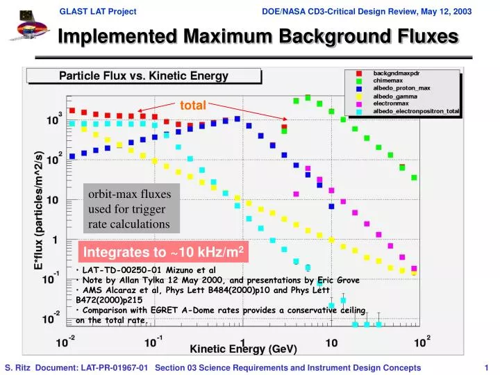
Implemented Maximum Background Fluxes total orbit-max fluxes used for trigger rate calculations Integrates to ~10 kHz/m2 • LAT-TD-00250-01 Mizuno et al • Note by Allan Tylka 12 May 2000, and presentations by Eric Grove • AMS Alcaraz et al, Phys Lett B484(2000)p10 and Phys Lett B472(2000)p215 • Comparison with EGRET A-Dome rates provides a conservative ceiling on the total rate.
Implemented Average Background Fluxes Integrates to ~4.2 kHz/m2 orbit-avg fluxes used for downlink and final background rejection calculations
EGRET A-dome Rates (from D. Bertsch, EGRET team) A-dome has an area of ~6 m2, so orbit max rate (outside SAA and no solar flares) corresponds to ~16 kHz/m2 This represents a conservative upper-limit for us, since the A-dome was sensitive down to 10’s of keV. Note peak rate is at (24.7,260) SAA
x x x • CAL: LO – independent check on TKR trigger. HI – indicates high energy event disengage use of ACD. Instrument Triggering and Onboard Data Flow Level 1 Trigger On-board Processing Hardware trigger based on special signals from each tower; initiates readout Function: • “did anything happen?” • keep as simple as possible full instrument information available to processors. Function: reduce data to fit within downlink Hierarchical filter process: first make the simple selections that require little CPU and data unpacking. • complete event information • signal/bkgd tunable, depending on analysis cuts: :cosmic-rays~ 1:~few • • subset of full background rejection analysis, with loose cuts • only use quantities that • are simple and robust • do not require application of sensor calibration constants • TKR 3 x•y pair planes in a row workhorse gtrigger OR Total L3T Rate: <25-30* Hz> (average event size: ~8-10* kbits) Upon a L1T, all towers are read out within 20ms On-board science analysis: transient detection (AGN flares, bursts) Instrument Total L1T Rate: <4 kHz>** Spacecraft **4 kHz average without throttle (1.3 kHz with throttle); peak L1T rate is approximately 12 kHz without throttle and 3.8 kHz with throttle). *assumes no compression
LOCAL • at least 2 methods to measure: • spatial distributions of L1T’s • compare TKR hits with TKR trigger pattern using both • TKR triggers • CAL-LO triggers (independent sample!) GLOBAL example: global trigger drops every 10th trigger. How would we know? Two types of global inefficiencies: Time-dependent monitor pulsar fluxes over time • Constant • At least 3 methods to measure: • count prescales • periodic triggers (both hard and soft) • use a sensor with a counter independent of trigger system (e.g., ACD tile) to generate heavily prescaled triggers. Testing Trigger Efficiencies On Orbit Two kinds of inefficiencies Test this on the ground in LAT using cosmic-ray induced muons