Download
1 / 30
300 likes | 462 Views
Vehicle Speed from Aerial Photography: Accuracy Analysis. Prof. Ismat M. Elhassan King Saud University Riyadh, Saudi Arabia E-mail: ismat@ksu.edu.sa. Presentation. Introduction Importance of Vehicle Speed Effects of Vehicle Speed Techniques of Vehicle Speed Determination

E N D
Vehicle Speed from AerialPhotography: Accuracy Analysis Prof. Ismat M. Elhassan King Saud University Riyadh, Saudi Arabia E-mail: ismat@ksu.edu.sa
Presentation Introduction Importance of Vehicle Speed Effects of Vehicle Speed Techniques of Vehicle Speed Determination Vehicle Speed from Aerial Photography Previous Studies Accuracy Analysis Conclusions
Introduction Definition: Speed is defined as the rate of motion (distance per unit of time). * Mathematically, speed or velocity, v is given by: v = d / t Where d is distance traveled during a unit time t * Speed of different vehicles will vary with respect to time and space.
Importance of Vehicle Speed *A basic measure of traffic performance and road safety * Establishing speed limits, * Determining safe speed limits at curves, * Establishing lengths of non-passing zones, * Location of traffic signals, * School or hospital zone protection, * Geometric design features: lengths of speed change lines, sight distance evaluation.
Effects of Vehicle Speed * Crashes of all types: - According to NHTSA’s 2011 Fatality Analysis Reporting System , high vehicle speed was a contributing factor in 29 % of all fatal crashes in USA. - In 2011, 32,367 people died in motor vehicle traffic crashes in the USA. - In 2011, an estimated 2.22 million people were injured in motor vehicle traffic crashes.
Car Accidents and Fatality in KSA According to A. Al-Ghamdi (1996):
Increase of Distance to Stop a Vehicle High Speed increases distance needed to stop a vehicle
Increasing Crash Energy * Increase in speed leads to exponential increase of crash energy: a 50% increase in speed causes impact energy to increase by 125% * A pedestrian hit at 64.4 km/h has an 85-percent chance of being killed; at 48.3 km/h the likelihood goes down to 45 percent, while at 32.2 km/h, the fatality rate is only 5 percent (U.K. Department of Transport).
Increasing Fatality Risk The fatality rate of pedestrians in crashes with passenger cars as function of the collision speed (Rosén et al., 2011).
Increasing Crash Frequency Traffic Speed and Crash Frequency
Techniques for Measuring Vehicle Speed RADAR: Shift in Frequency by Doppler Effect Sources of Errors: Cosine error, frequency drift due to temp change and volt fluctuation. Radar units must be calibrated.
LIDAR Speed Detector LIDAR : LIghtDetection And Ranging. A police laser emits a highly focused beam of invisible light, in the near infrared region of light, that is centered at 904nm of wavelength and is only about 56cm in diameter at 300m. Police laser-lidarcalculates speed by observing the changing amount of time it takes to "see" reflected pulses of light over a discreet amount of time.
GPS GPS devices are positional speedometers. GPS algorithm also uses the Doppler shift in the pseudo range signals from the satellites. It should also be noted that the speed reading is normalized, and is not an instant speed. Accuracy of calculated speed, is dependent on the satellite signal quality at the time.
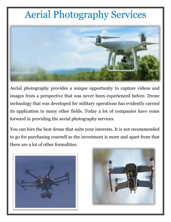
Overlapping Aerial Photographs Overlapping aerial photos allow capturing positions of moving vehicle at two different instants known as time interval of aerial Photos. Howes, William F and Miles, Robert Douglas, in 1963, published a technical paper titled: "Aerial Photography Applied to Traffic Studies" in report number FHWA/IN/JHRP-63/14, Purdue University, USA.
Speed from Digital Aerial Photography From: Fumio Yamazaki et al, 2007: Two consecutive aerial images of central Tokyo having about 3.08 s time lag, taken by digital aerial camera. The images were provided by Geographical Survey Institute of Japan.
Continuous Strip Aerial Photography In 1965 McCasland reported on comparison of two techniques of aerial photography for application in freeway traffic operation studies: using aerial strip photography (ASP) and aerial time lapse photography. ASP provided more coverage while more speed readings can be given by time lapse photography.
Aerial Video PituMirchandani, et. al, 2002 reported on aerial video application on traffic performance. The estimated speeds of the matched vehicles were calculated using the image scale and the time between frames. Vehicle speeds were fairly well clustered around 48-53 mph, as one might expect along a freeway. The lone exception was vehicle 9 which had an observed speed of over 70 mph. This anomalous speed was due to the erroneous matching of vehicle 9 with vehicle 10. Such an erroneous speed could be discovered by a simple filter.
Satellite Imagery Zhang and Xiong (2006) and presented a technique to detect a moving vehicle using one single set (Panch. and MSS sensors)of Quickbird imagery. The test results showed that the position, speed and moving direction of a vehicle can be determined at a reasonable accuracy. The speed accuracy depends on the image resolution, accuracy of vehicle image coordinates and accuracy of satellite time interval between Panchromatic and Multispectral images.
Photogrammetric Approach The overlapping photos method: Assuming time lapse between the overlapping photographs is t (seconds), image distance between the positions of the vehicle on one of the photographs is measured as: d (mm), flying height H and camera focal length f, are given in meters and mms, respectively: vehicle speed, v = (d*H/f) / (t) m/sec
Time lapse Overlapping photography Two aerial photos exposed from stations O1 and O2: O1 O2 f c1 c1 c2 H C1 C2 Car position C1 moved to positionC2 during time lapse between photos
Vehicle speed formula The vehicle speed v (m/s) can be calculated from the time-distance relation: v = D / t, or v = d (H/f)/ t, where t is the time interval between the consecutive photos in seconds. To determine the speed in kilometers per hour: v = d (H/f)/ t * (3600/1000) or: v = 3.6 * d (H/f)/ t
Variance of computed speed Given a function F(x,y) in wich both arguments x and y contain statistical errors and are statistically independent, the variance for the value of F(x,y) is obtained by law of propogation of errors: var(F) = (∂F/∂x)2var(x) + (∂F/∂y)2var(y). Stand. Error: dF = var(F(x,y))1/2. This law is applied to determine error in car speed:
Standard Errorin Vehicle Speed The function, F, is the vehicle speed, v. The standard error in v will be given as: dv = var(v(d, H, f, t ))1/2. var(v) = (∂v/∂d)2var(d) + (∂v/∂H)2var(H) + (∂v/∂f)2var(f) + (∂v/∂t)2var(t) Where: ∂v/∂d = 3.6(H/f) / t, ∂v/∂H =3.6 (d/f) / t, ∂v/∂f = 3.6 * [d (H)/ t] / (f2), ∂v/∂t= [3.6 * d (H/f)] / (t)2
Tested Data - 1 DATA 1: Vehicle speed v = 50 km/h, 100km/h, 150km/h Photo scale: 1/5000, t = 5 sec. σd = 0.01mm Effect of change in σt (accuracy of time interval) Results:
Errors in v scale 1:5000 Sigma v Sigma dt dt= 5 sec, Sigma d=0.01mm, v1=50k/h, v2=100;/h, v3=150k/h, standard error in k/h 50k/h 100k/h 150k/h
Test Data - 2 DATA 2: Vehicle speed v = 50 km/h, 100km/h, 150km/h Photo scale: 1/10000, t = 5 sec. σd = 0.01mm Results:
Test Data - 3 DATA 3: Vehicle speed v = 50 km/h, 100km/h, 150km/h Photo scale: 1/5000, t = 5 sec. σd = 0.01mm Effect of change in σd (accuracy of mesuring vehicle movement on photo), Results:
Graphical Representation Effect of change in sigma d and scale
Conclusions • From the above tests and results it can be concluded that: • *To get high vehicle speed accuracy we need to have: • Highly accurate measured time interval between photos (intervalometer) • Highly accurate photo measured distance moved by vehicle. • Large scale photography * The advantage of using aerial photography is that the information is available any time needed.
END • THANKS • For all audience • Have good time