Download
1 / 22
220 likes | 288 Views
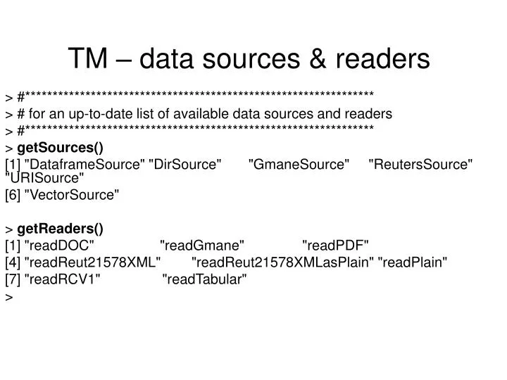
TM – data sources & readers. > #**************************************************************** > # for an up-to-date list of available data sources and readers > #**************************************************************** > getSources()

E N D
TM – data sources & readers > #**************************************************************** > # for an up-to-date list of available data sources and readers > #**************************************************************** > getSources() [1] "DataframeSource" "DirSource" "GmaneSource" "ReutersSource" "URISource" [6] "VectorSource" > getReaders() [1] "readDOC" "readGmane" "readPDF" [4] "readReut21578XML" "readReut21578XMLasPlain" "readPlain" [7] "readRCV1" "readTabular" >
TM – source documents #**************************************************************** # read in source document collection #**************************************************************** >txt.csv <- read.csv(file="c:/text mining/Top2Iss.txt", header=FALSE) >txt <- Corpus(DataframeSource(txt.csv)) >summary(txt) A corpus with 330 text documents # examine the first 10 rows >inspect(txt[1:10]) [[1]] A crisis that could affect our ability to regulate ourselves. [[2]] A need to deal more thoroughly with non-traditional risk management approaches [[3]] Ability of members to prove they are more than just number crunchers [[4]] ability to convince non-insurance companies of the value/skills offered by CAS members.
TM – preprocess - lowercase > #**************************************************************** > # a little pre-processing to prep the data for TM > # convert to lower case > # tmTolower is one of several available text transformations. > # To see all currently available use: getTransformations() > #**************************************************************** > txt <- tm_map(txt, tolower) > inspect(txt[1:10]) [[1]] a crisis that could affect our ability to regulate ourselves. [[2]] a need to deal more thoroughly with non-traditional risk management approaches [[3]] ability of members to prove they are more than just number crunchers [[4]] ability to convince non-insurance companies of the value/skills offered by cas members.
TM – search & replace > #**************************************************************** > # Replace the slashes in the text with a blank > #**************************************************************** > # txt <- gsub("/"," ",txt) for (j in 1:length(txt)) txt[[j]] <- gsub("/", " ",txt[[j]]) > inspect(txt[1:10]) [[1]] a crisis that could affect our ability to regulate ourselves. [[2]] a need to deal more thoroughly with non-traditional risk management approaches [[3]] ability of members to prove they are more than just number crunchers [[4]] ability to convince non-insurance companies of the value skills offered by cas members.
TM – search & replace con’t > #**************************************************************** > # Replace other characters > #**************************************************************** > > for (j in 1:length(txt)) txt[[j]] <- gsub("[&-/\\()\\.]", " ",txt[[j]]) > for (j in 1:length(txt)) txt[[j]] <- gsub("[|&|-|/|\\|()|\\.]", " ", txt[[j]]); > inspect(txt[1:10]) [[1]] a crisis that could affect our ability to regulate ourselves [[2]] a need to deal more thoroughly with non traditional risk management approaches [[3]] ability of members to prove they are more than just number crunchers [[4]] ability to convince non insurance companies of the value skills offered by cas members [[5]] ability to help sort out property pricing problems
TM – search & replace con’t > #**************************************************************** > # Replace enterprise risk management > #**************************************************************** > for (j in 1:length(txt)) txt[[j]] <- gsub("enterprise risk management", "erm",txt[[j]]) > for (j in 1:length(txt)) txt[[j]] <- gsub("off shoring", "offshoring", txt[[j]]); > inspect(txt[1:10]) [[1]] a crisis that could affect our ability to regulate ourselves [[2]] a need to deal more thoroughly with non traditional risk management approaches [[3]] ability of members to prove they are more than just number crunchers [[4]] ability to convince non insurance companies of the value skills offered by cas members [[5]] ability to help sort out property pricing problems
TM – search & replace con’t • > #**************************************************************** • > # remove stopwords • > #**************************************************************** • > txt <- tm_map(txt, removeWords, stopwords("english")) • > #dbInit(db='txtcsv') • > • > #**************************************************************** • > # remove punctuation • > #**************************************************************** • > txt <- tm_map(txt, removeNumbers) • > txt <- tm_map(txt, removePunctuation) • > inspect(txt[1:10]) • [[1]] • crisis affect ability regulate • [[2]] • deal thoroughly traditional risk management approaches • [[3]] • ability prove crunchers • [[4]] • ability convince insurance companies value skills offered cas • [[5]] • ability help sort property pricing
TM – search & replace con’t • > #**************************************************************** • > # remove stopwords & punctuation • > #**************************************************************** • > txt <- tm_map(txt, removeWords, stopwords("english")) • > txt <- tm_map(txt, removeNumbers) • > txt <- tm_map(txt, removePunctuation) • > inspect(txt[1:10]) • [[1]] • crisis affect ability regulate • [[2]] • deal thoroughly traditional risk management approaches • [[3]] • ability prove crunchers • [[4]] • ability convince insurance companies value skills offered cas • [[5]] • ability help sort property pricing • > length(txt); • [1] 330
TM – search & replace con’t (j in 1:length(txt)) txt[[j]] <- gsub("professional", "professions", txt[[j]]); > > getTransformations() [1] "as.PlainTextDocument" "convert_UTF_8" "removeNumbers" "removePunctuation" [5] "removeWords" "stemDocument" "stripWhitespace" > txt <- tm_map(txt, stemDocument) > inspect(txt[40:50]) [[1]] climat chang [[2]] compani complain oner expen educ system set cas [[3]] compani will pay meet [[4]] compet profess organ [[5]] competit profess
TM – Document by Term Matrix > #**************************************************************** > # create a document_by_term matrix > #**************************************************************** > dtm <- DocumentTermMatrix(txt) > nrow(dtm); ncol(dtm) [1] 330 [1] 469 > inspect(dtm[1:24,1:9]) A document-term matrix (24 documents, 9 terms) Non-/sparse entries: 10/206 Sparsity : 95% Maximal term length: 8 Weighting : term frequency (tf) abil aca accept account accredit accuraci activ actuari address 1 1 0 0 0 0 0 0 0 0 2 0 0 0 0 0 0 0 0 0 3 1 0 0 0 0 0 0 0 0 4 1 0 0 0 0 0 0 0 0 5 1 0 0 0 0 0 0 0 0 6 0 0 1 0 0 0 0 0 0 7 0 0 0 0 0 0 0 1 0 8 0 0 0 0 0 0 0 1 0 9 0 0 0 0 0 0 0 1 0 10 0 0 0 0 0 0 0 0 0
TM – ID Frequent Occuring Words > #**************************************************************** > # ID frequently occuring words > #**************************************************************** > findFreqTerms(dtm, 1.2)# 2 occurances=lower frequency bound; [1] "exam" "cost" "smart" "actuari" "focus" "expen" "profess" > > #**************************************************************** > # tighten up dtm matrix by removing sparse terms > #**************************************************************** > nrow(dtm); ncol(dtm) [1] 330 [1] 469 > dtm2 <- removeSparseTerms(dtm, 0.995) > nrow(dtm2); ncol(dtm2) [1] 330 [1] 192 > inspect(dtm2[1:12,1:15]) abil aca accept account activ actuari admiss aig analysi analyst analyt applic approach 1 1 0 0 0 0 0 0 0 0 0 0 0 0 2 0 0 0 0 0 0 0 0 0 0 0 0 1 3 1 0 0 0 0 0 0 0 0 0 0 0 0 4 1 0 0 0 0 0 0 0 0 0 0 0 0 5 1 0 0 0 0 0 0 0 0 0 0 0 0 6 0 0 1 0 0 0 0 0 0 0 0 0 0 7 0 0 0 0 0 1 0 0 0 0 0 0 0 8 0 0 0 0 0 1 0 0 0 0 0 0 0 9 0 0 0 0 0 1 0 0 0 0 0 0 0 10 0 0 0 0 0 0 1 0 0 0 0 0 0
TM – Remove Sparse terms > #**************************************************************** > # tighten up dtm matrix more for correlation plot by removing sparse terms > #**************************************************************** > dtm3 <- removeSparseTerms(dtm, 0.98) > nrow(dtm3); ncol(dtm3) [1] 330 [1] 36 > #inspect(dtm3[1:3,]) > > findFreqTerms(dtm3, 2) [1] "exam" "actuari" "focus" "profess" > > # find words correlated with the themes > findAssocs(dtm2, "educ", 0.05) educ regard system train topic research practic qualiti 1.00 0.37 0.37 0.37 0.25 0.23 0.20 0.20 continu environ materi pressur set syllabus current applic 0.18 0.18 0.18 0.18 0.18 0.14 0.13 0.11 opportun reput result student provid actuari exam expen 0.11 0.11 0.11 0.11 0.10 0.09 0.09 0.09 chang structur casualti membership relev 0.08 0.08 0.06 0.06 0.06
TM – Find Frequent terms ************************************************************** > # export dtm > #**************************************************************** > top2.matrix <- as.matrix(dtm3) > write.csv(top2.matrix, file="c:/text mining/top2tf.csv", row.names=FALSE) ********************************************************* > # find most frequently mentioned terms > #**************************************************************** > tags <- sort(findFreqTerms(dtm3, 1, 3)); tags[1:10] [1] "abil" "account" "actuari" "cas" "casualti" "chang" "compani" "competit" [9] "continu" "credibl" > #tags <- sort(paste('top2$',findFreqTerms(dtm2, 1, 3),sep="")); tags[1:10] > sum(abil); # returns 5 [1] 7 > sum(actuari); # returns 60 [1] 62 > sum(account); # returns 6 [1] 8 > numwords <- 30 > v <- as.matrix(sort(sapply(top2, sum),decreasing=TRUE)[1:numwords], colnames=count);v[1:numwords] [1] 62 33 23 20 19 17 15 15 14 14 14 14 12 12 12 12 11 11 11 11 10 10 10 10 9 9 9 9 8 8 > w <- rownames(v); length(w); w [1] 30 [1] "actuari" "profess" "insur" "financ" "chang" "erm" "exam" "regul" [9] "cas" "competit" "educ" "increa" "compani" "credibl" "intern" "model" [17] "current" "organ" "reserv" "standard" "focus" "industri" "manag" "research" [25] "global" "issu" "market" "risk" "account" "casualti" > require(grDevices); # for colors > x <- sort(v[1:10,], decreasing=FALSE) > barplot(x, horiz=TRUE, cex.names=0.75, space=1, las=1, col=grey.colors(10), main="Frequency of Terms") >
barplot(x, horiz=TRUE, cex.names=0.75, space=1, las=1, col=grey.colors(10), main="Frequency of Terms")
Three Variations on Tag Clouds #************************************************************** # tag Cloud as a list 2/06/Tag-cloud-for-the-R-Graph-Gallery #**************************************************************# as a list require(snippets) v <- sapply(top2, sum);v cloud(v, col=col.bbr(v, fit=TRUE))
Three Variations on Tag Clouds #****************************************** # Tag Cloud with random placement #****************************************** set.seed(221); factor=0.8; x=runif(length(w))*factor; y=runif(length(w))*factor; plot(x, y, type="n", axes=FALSE); # font size=relative term frequency pointLabel(x, y, w, 0.10*v);
Three Variations on Tag Clouds #**************************************************************** # install.packages("fun", repos="http://r-forge.r-project.org"). # with style #**************************************************************** require(fun) data(tagData) v <- as.matrix(sort(sapply(top2, doit),decreasing=TRUE)[1:numwords], colnames=count);v[1:numwords];v x <-data.frame(rownames(v), "http://www.casact.org/", v, tagData$color[1:length(v)],tagData$hicolor[1:length(v)]); colnames(x) <- c('tag','link', 'count','color','hicolor');x htmlFile=paste(tempfile(), ".html", sep="") #htmlFile=paste("tagData", ".html", sep="") if (file.create(htmlFile)) { tagCloud(x, htmlFile) browseURL(htmlFile) }
Get Individual Records associated with the term “actuar” > #**************************************************************** > # Get records for the word actuar > #**************************************************************** > subset(top2, actuari>=1)[1:10,1:10] abil account actuari cas casualti chang compani competit continu credibl 7 0 0 1 0 0 0 0 0 0 0 8 0 0 1 0 0 0 0 0 0 0 9 0 0 1 0 0 0 0 0 0 0 17 0 0 1 0 0 0 0 0 0 0 > rownames(subset(top2, actuari>=1)) #which rows have actauri=1 [1] "7" "8" "9" "17" "20" "45" "46" "57" "59" "71" "74" "77" "78" "81" [15] "82" "95" "105" "118" "136" "149" "153" "160" "163" "173" "180" "182" "183" "186" [29] "191" "193" "195" "196" "197" "204" "205" "206" "214" "220" "221" "223" "224" "225" [43] "227" "229" "250" "261" "263" "266" "277" "282" "298" "299" "309" "313" "318" "321" [57] "323" "328" "329" > txt.actuari <- txt.csv[rownames(subset(top2, actuari>=1)),] > txt.actuari[1:5]; #print out records with actuari [1] Actuarial Malpractice (2) [2] Actuarial Students of today are not good communicators/executive material. [3] Actuaries regain status as masters of risk [4] automation/modeling of actuarial skills [5] Being a market leading brand of actuarial science - what do we stand for? 330 Levels: approaches to address external changes ERM ... Will we get to a point where we have too many members??
Correlation Plot > #**************************************************************** > # produce a Correlation plot with the most frequenctly occuring top 24 terms > #**************************************************************** > require(ellipse) > nrow(dtm3); ncol(dtm3) [1] 330 [1] 36 > dtm4 <- removeSparseTerms(dtm, 0.97) > nrow(dtm4); ncol(dtm4) [1] 330 [1] 23 > inspect(dtm4[1:3,]) actuari cas chang compani competit credibl current educ erm exam financ increa industri 1 0 0 0 0 0 0 0 0 0 0 0 0 0 2 0 0 0 0 0 0 0 0 0 0 0 0 0 3 0 0 0 0 0 0 0 0 0 0 0 0 0 insur intern manag model organ profess regul research reserv standard 1 0 0 0 0 0 0 1 0 0 0 2 0 0 1 0 0 0 0 0 0 0 3 0 0 0 0 0 0 0 0 0 0 > top4.matrix <- as.matrix(dtm4) > txt.corr <- cor(top4.matrix) > ord <- order(txt.corr[ncol(dtm4),]) > xc <- txt.corr[ord, ord] > plotcorr(xc, col=cm.colors(12)[5*xc + 6]) >
******************************************************* > # hierarchical clustering (Ward's minimum variance method) > #************************************************************************ > require(stats) > #new for clustering variables > dtm3 <- removeSparseTerms(dtm, 0.97) > dtmtrans<-t(dtm3) > hClust <- hclust(dist(dtmtrans), method='ward'); # average, single, complete, median, centroid, ward, mcquitty; > plot(hClust) > # for interactive plot > # (x <- identify(hClust)) > > require(graphics); > require(utils) > (dend1 <- as.dendrogram(hClust)) # "print()" method 'dendrogram' with 2 branches and 23 members total, at height 12.07791 > dend2 <- str(dend1, max=4) # only the first two sub-levels --[dendrogram w/ 2 branches and 23 members at h = 12.1] |--leaf "actuari" `--[dendrogram w/ 2 branches and 22 members at h = 8.3] |--leaf "profess" `--[dendrogram w/ 2 branches and 21 members at h = 6.48] |--[dendrogram w/ 2 branches and 2 members at h = 6.08] | |--leaf "financ" | `--leaf "insur" `--[dendrogram w/ 2 branches and 19 members at h = 6.15] |--[dendrogram w/ 2 branches and 2 members at h = 5.66] .. `--[dendrogram w/ 2 branches and 17 members at h = 5.78] .. > plot(dend1) Correlation Plot