Download
1 / 55
550 likes | 719 Views
Network Flows. Minimum-Cost Flow Problems (Section 6.1) 6.2–6.12 A Case Study: The BMZ Maximum Flow Problem (Section 6.2) 6.13–6.16 Maximum Flow Problems (Section 6.3) 6.17–6.21 Shortest Path Problems: Littletown Fire Department (Section 6.4) 6.22–6.25

E N D
Minimum-Cost Flow Problems (Section 6.1) 6.2–6.12 A Case Study: The BMZ Maximum Flow Problem (Section 6.2) 6.13–6.16 Maximum Flow Problems (Section 6.3) 6.17–6.21 Shortest Path Problems: Littletown Fire Department (Section 6.4) 6.22–6.25 Shortest Path Problems: General Characteristics (Section 6.4) 6.26–6.27 Shortest Path Problems: Minimizing Sarah’s Total Cost (Section 6.4) 6.28–6.31 Shortest Path Problems: Minimizing Quick’s Total Time (Section 6.4) 6.32–6.36 Table of ContentsChapter 6 (Network Optimization Problems)
Distribution Unlimited Co. Problem • The Distribution Unlimited Co. has two factories producing a product that needs to be shipped to two warehouses • Factory 1 produces 80 units. • Factory 2 produces 70 units. • Warehouse 1 needs 60 units. • Warehouse 2 needs 90 units. • There are rail links directly from Factory 1 to Warehouse 1 and Factory 2 to Warehouse 2. • Independent truckers are available to ship up to 50 units from each factory to the distribution center, and then 50 units from the distribution center to each warehouse. Question: How many units (truckloads) should be shipped along each shipping lane?
Minimum Cost Flow Problem: Narrative representation There are 2 plants, 2 demand centers and 1 transshipment point. Production of Plants 1 and 2 are 80 and 70 units respectively. Demand of Demand centers 1 and 2 ( we call them points 4 and 5) are 60 and 90 units respectively. Transshipment point ( point 3) is does not have any supply or demand. Given the information on the next page, formulate this problem as an LP to satisfy supply and demand with minimal transportation costs.
Minimum Cost Flow Problem: Narrative representation Transportation costs for each unit of product and max capacity of each road is given below From To cost/ unit Max capacity 1 4 700 No limit 1 3 300 50 2 3 400 50 2 5 900 No limit 3 4 200 50 3 5 400 50 There is no other link between any pair of points
Minimum Cost Problem: Pictorial Representation x14 30 80 1 4 60 x13 x34 50 30 50 50 3 30 50 50 50 x23 x35 x25 40 70 2 5 90
Conventions Minimum Cost Flow is the same as Transportation and Transshipment problem. We reformulate the same problem in the context of Minimum Cost flow just as an introduction to the domain of the Network Optimization Problems. For each node i , we define the net flow as the difference between total outflow minus total inflow. fi : Net flow of node i If i is asupplypointthenfi= + supply of nodei If i is ademandpointthenfi= - demand of nodei If i is atransshipment pointthenfi= 0
Notations and Formulation Notation tij : Outflow from node i to node j withi --------->j tji : Inflow from node j to node i withi<----------j Tij : Maximum capacity of arcij tij Tij ij A ( A is the setof directed arcs) fi : Net flow of node i tij - tji = fi i N ( N is the set of nodes) cij : Cost of moving one unit on arcij
Minimum Cost Flow Problem: decision variables x14 = Volume of product sent from point 1 to 4 x13 = Volume of product sent from point 1 to 3 x23 = Volume of product sent from point 2 to 3 x25 = Volume of product sent from point 2 to 5 x34 = Volume of product sent from point 3 to 4 x35 = Volume of product sent from point 3 to 5 We want to minimize Z = 700 x14 +300 x13 + 400 x23 + 900 x25 +200 x34 + 400 x35
Minimum Cost Flow Problem: constraints Supply x14 + x13 = 80 x23 + x25 = 70 Demand x14 + x34 = 60 x25 + x35 = 90 Transshipment x13 + x23 = x34 + x35 (Move all variables to LHS) x13 + x23 - x34 - x35 =0
Minimum Cost Flow Problem: constraints Capacity x13 50 x23 50 x34 50 x35 50 Nonnegativity x14, x13 , x23 , x25 , x34 , x35 0
700 80 1 4 -60 300 200 50 50 3 400 400 50 50 900 70 2 5 -90 Example Node 1 : t13 + t14 = 80 ( the same for node 2) Node 4 : -t14 - t34 = -60 (the same for node 5) Node 3 : t34 + t35 -t13 - t23 = 0 Capacity Constraints on arc 13 : t13 50( the same for arcs 2-3, 3-4, and 3-5) Min Z = + 300 t13 + 700 t14 + 400 t23 + 900 t25 + 200 t34 + 400 t35
700 80 1 4 -60 300 200 50 50 3 400 400 50 50 900 70 2 5 -90 Excel
Minimum Cost Problem: Pictorial Representation 30 80 1 4 60 50 30 50 50 3 30 50 50 50 40 70 2 5 90
900 +50 -30 400 300 200 50 200 300 80 100 +40 -60 Transportation problem III : Pictorial representation x14 1 4 x13 x12 3 x35 x54 x45 x23 2 5
Transportation problem III : Formulation Material Flow Balance. At each node we have Supply + Inflow = Demand + Outflow 50 = x12+ x13 + x14 40+x12 = x23 x13+ x23 = x35 x14+ x54 = 30 + x45 x35+ x45 = 60 + x54 Capacity x12 50 x35 80 Min Z = 200x12+ 400x13 +900x14 +300x23 +100x35 + 300x45 + 200x54
60 80 50 40 70 5 4 6 D 2 O 3 70 50 40 30 The Maximum Flow Problem There is no inflow associated with origin There is no outflow associated with destination We want to Maximize total outflow of the origin or total inflow of the destination
Notations and Formulation tij : Outflow from node i to node j withi --------->j tji : Inflow from node j to node i withi <----------j Tij : Maximum capacity of arcij tij Tij ij A fi : iszerofor all nodesexcept Origin(s) and Destination(s) tij - tji = 0 i N \ O and D
60 80 50 40 70 D 6 3 2 5 O 4 70 50 40 30 Example t25 - tO2 = 0 t35 + t36 -tO3 = 0 t46 - tO4 = 0 t5D - t25 -t35 = 0 t6D - t36 -t46 = 0 tO2 50 tO3 70 tO4 40 t25 60 t35 40 t36 50 and so on t6D 70 Max Z = tO2 + tO3 +tO4
60 80 50 40 70 5 3 6 O 2 D 4 70 50 40 30 Excel and Solver
O 5 4 3 2 6 D 60(50) 80 50 40 (30) 70 70 50(40) 40 (30) 30 Solution
7 40 8 60 20 30 10 20 D2 O2 60 40 80 50 40 6 2 3 4 5 D1 70 O1 40 70 50 30 More Than One Origin tij - tji = 0 i N \ Os and Ds tij Tij ij A
7 40 8 60 20 30 10 20 D2 O2 D 4 5 2 6 3 60 40 40 80 50 40 70 O1 70 50 30 Example tij - tji = 0 i N \ Os and Ds Example: Node 7 + t78 + t75 -tO27 = 0 Example: Node 5 + t5D1 + t5D2 -t25 -t35 -t75 = 0 tij Tij ij A Example: Arc 46 t46 30 Example: Arc O12 tO12 50 Objective Function Max Z = + tO12 + tO13 + tO14 + tO22 + tO27
The Shortest Route Problem The shortest route between two points l ij : The length of the directed arc ij. l ij is a parameter, not a decision variable. It could be the length in term ofdistance or in terms of time or cost ( the same asc ij ) For those nodes which we are sure that we go from i to jweonly have one directed arc from i to j. For those node which we are not sure that we go from i to j or from j to i, we have two directed arcs, one from i to j, the other from j to i. We may have symmetric or asymmetric network. In a symmetric networklij = lji ij In a asymmetric networkthis condition does not hold
Example 2 6 6 5 2 2 4 2 7 6 1 4 2 8 2 5 2 7 3
Decision Variables and Formulation xij : The decision variable for the directed arc from node i to nod j. xij = 1 if arc ij is on the shortest route xij = 0 if arc ij is not on the shortest route xij - xji = 0 i N \ O and D xoj =1 xiD = 1 Min Z = lij xij
Example 2 6 6 5 2 2 4 2 7 6 1 4 2 8 2 5 2 7 3
6 6 3 4 2 5 2 2 5 4 2 2 6 7 1 2 8 2 7 Example + x13 + x14+ x12= 1 - x57 - x67= -1 + x34 + x35 - x43 - x13 = 0 + x42 + x43 + x45 + x46 - x14 - x24 - x34 = 0 …. ….. Min Z = + 5x12 + 4x13 + 3x14 + 2x24 + 6x26 + 2x34 + 3x35 + 2x43 + 2x42 + 5x45 + 4x46 + 3x56 + 2x57 + 3x65 + 2x67
6 6 3 4 2 5 2 2 5 4 2 2 6 7 1 2 8 2 7 Excel
6 6 3 4 2 5 2 2 5 4 2 2 6 7 1 2 8 2 7 Excel
6 2 2 5 4 2 6 7 1 2 8 2 2 7 2 4 3 6 5 Solver Solution
6 4 9 6 3 4 3 6 2 2 11 2 2 6 6 6 3 7 4 8 5 2 2 5 4 3 5 4 3 3 10 1 2 5 2 3 D O After class practice; Find the shortest route
2 1 3 4 6 1 2 3 4 Two important observations in the LP-relaxation Formulate on the problem on the black board Did I say xij <= 1 ? Why all the variables came out less than 1 Did I say xij 0 or 1 Why all variables came out 0 or 1
The Minimum Spanning Tree Find a tree such that we can access each and every node at the minimum cost. The total length ( or cost) of the tree is minimized. In other words, we want to minimize the construction cost of the tree. Edges on the MST are bi-directional l ij : The length or cost of the bi-directional edge ij. We usually use the term “EDGE” as nondirected, and term “ARC” as directed. All distances in MSE network are symmetric.
7 2 2 5 4 7 2 4 3 5 1 6 5 3 4 1 1 7 4 The Minimum Spanning Tree
2 7 2 2 5 4 1 6 4 5 3 4 7 1 7 4 3 5 Minimum Spanning Tree
2 7 2 2 5 4 1 6 4 5 3 4 7 1 7 4 3 5 Minimum Spanning Tree
2 7 2 2 5 4 1 6 4 5 3 4 7 1 7 4 3 5 Minimum Spanning Tree : Connectivity
2 7 2 2 5 4 1 6 4 5 3 4 7 1 7 4 3 5 Minimum Spanning Tree : Connectivity
2 7 2 2 5 4 1 6 4 5 3 4 7 1 7 4 3 5 Minimum Spanning Tree : Integrality