Download
1 / 18
190 likes | 337 Views
Andrea Censi , Luca Iocchi, Giorgio Grisetti lastname @ dis.uniroma1.it www.dis.uniroma1.it/~ lastname. Scan matching in the Hough domain. SIED Lab www.dis.uniroma1.it/~multirob/sied/. Scan matching .

E N D
Andrea Censi, Luca Iocchi, Giorgio Grisetti lastname @ dis.uniroma1.it www.dis.uniroma1.it/~lastname Scan matching in the Hough domain SIED Lab www.dis.uniroma1.it/~multirob/sied/
Scan matching • 2D scan matching (geometric interpretation): find a rotation and a translation T who maximize overlapping of two sets of 2D data. • 2D scan matching (probabilistic interpretation): approximate a pdf of the robot pose; ex: p(xt|xt-1, ut-1, yt, yt-1)or others... Map portion Sensor scan
Previous research • Existing methods differ by: • assumptions about environment (ex: features?) • assumptions about sensing devices (noise, FOV) • assumptions about the search domain (local vs. “global”) • representation of uncertainty (multi-hypothesis, continuous pdf) • Methods performing a local search: • features based [ex: Guttman ‘96, Lingemann ‘04] • ICP family [Lu-Milios ‘94, several extensions/optimizations] • gradient-based iterative methods [ex: Hähnel ‘02, Biber ‘03] • Methods performing a global search: • feature based: many [ex: us, 2002] • histogram of surface angles [ex: Weiß ‘94] • extensive search: 2D correlation [Konolige-Chou ‘99]
Hough Scan Matching (HSM) • Our approach: • works in unstructured environments and with noisy range finders (we don’t do feature “detection”, we work with features “distributions”) • global search (but if a guess is available, it performs efficient local search) and multi-modality (detects ambiguities) • completeness: if an exact match exists, it will be included in the solution set (works in practice with very different data). • Algorithm. Given reference and sensor data: • compute the Hough Transform (HT) for both • compute the Hough Spectrum (HS) from the HT • find hypotheses for via the cross-correlation of the HS • given an estimate , estimate T via cross-correlation of the HT andrea: decoupling
7 - The Hough Transform (HT) • The simplest HT transforms the cartesian space X-Y into the Hough Domain (, ). The straight line cos()x+sin()y = r corresponds to point (, r) in the Hough Domain. Andrea Censi: si può fare in modo formale r HT r (x,y) cartesian plane Hough Domain (, )
7 - The Hough Transform (HT) • A point in the cartesian plane a sinusoid in the Hough domain • Sinusoids of collinear points intersects. Andrea Censi: si può fare in modo formale Hough Domain (, ) Cartesian plane (x,y).
Feature detection with the HT HT andrea: in you algorithm
Expressiveness of the HT HT HT-1 “features distributions”
Definition of Hough Spectrum HT[i] HT g HSg[i] • The spectrum is a a function of with 180° period. • We compute a “spectrum” from the Hough Transform (applying a translation-invariant functional g to the columns of the HT) i
Hough Spectrum properties T T (same spectrum) • it is invariant to input translation • it shifts on input rotation Andrea Censi: anche alla scala
HSM: finding the rotation HSg[i] HSg[i’] cross correlation +180° The peaks of the cross correlation are estimates for . • The spectrum of an input transformed by (,Tx,Ty) is shifted by regardless of T; we can estimate by correlating the two spectra. T
Handling ambiguities • Multi-modal global search can detect ambiguities multiple hypotheses for Input data Hough spectrum result of correlation
Comparison with circular histogram result of correlation Input data histogram of surface angles Hough spectrum The histogram of surface angles has similar properties, but • HS works with noisier data (does not need orientation information) • HS can handle cases when the circular histogram fails. Example: Andrea Censi: anche alla scala
HSM: estimating T translation T T HT HT |T|
HSM: how to estimate T linear constraints d d' T d' ~ p(T| ) d • Given an estimate of , we can get linear constraints for T comparing columns of the HT (“directions of alignment”). We choose the directions with higher expected energy = peaks of the spectrum. T
Example with real data First solution (exact) Second solution Map portion Laser scan
Summary • Operating in the Hough space allows to decouple the search of the rotation from the translation (3D search 3 x 1D searches ) • Does not rely on the existence of features. • Multi-modal and global search (efficient local search). • Experimental simulation results: • Good results in curved enviroments if sensor is accurate. • Reliability to different kinds of sensor noise (except for high discretization). • Future (hard) work: extension to 3D for dealing with 3D noisy sensors (stereo camera).
Thanks for your attention • Slides and an extended version of the paper available at www.dis.uniroma1.it/~censi Andrea Censi, Luca Iocchi, Giorgio Grisetti lastname @ dis.uniroma1.it www.dis.uniroma1.it/~lastname