Download
1 / 77
820 likes | 1.1k Views
David H. Ardell,Forskarassistent. Introduction to Evolutionary Bioinformatics. Outline, v. 4. Wed. Jan. 26 Sequences and substitution matrices. Thurs. Jan. 27 Alignments: basic theory and practice. Fri. Jan. 28 Trees: basic theory and practice.

E N D
David H. Ardell,Forskarassistent Introduction to Evolutionary Bioinformatics
Outline, v. 4 • Wed. Jan. 26 Sequences and substitution matrices. • Thurs. Jan. 27 Alignments: basic theory and practice. • Fri. Jan. 28 Trees: basic theory and practice. • Mon. Jan. 31 Population sequence data: theory and practice.
Lecture Outline: Intro. to Sequence Evolution and Substitution Matrices • Part I: Theory • Homology, paralogy and orthology • Molecular clock • Divergence, saturation and evolutionary distance • Poisson correction • PAM and other substitution matrices • Markov and other assumptions of bioinformatics • Sequence compositions • Part II: Practice • Evolving sequences on a computer • Calculating evolutionary distances • Exploring Substitution matrices • Calculating evolutionary distance with substitution matrices
Richard Owen (1804-1892) HOMOLOGY: descent from a common ancestor(Darwin, 1859) Original definition: "the same organ in different animals under every variety of form and function." (Owen, 1843). Homology need not imply similarity of form nor function because of divergence. Similarity need not imply homology because of convergence.
Homology applied to DNA sequences: Ancestralsequence GCCACTTTCGCGATCA GCCACTTTCGCGATCA GCCACTTTCGCGATCG GCCACTTTCGCGATTA GCCACTTTCGTGATCG GCCACGTTCGTGATCG GACAGTTTCGCGATTA GCCACGTTCGCGATCG Homologous sequences GGCAGTTTTGCGATTA GCCACGTTCGCGATCG GGCAGTTTCGCGATTT GGCAGTTTCGCGATTT GCCACGTTCGCGATCG GCCACGTTCGCGATCG | || ||||||| GGCAGTCTCGCGATTT Homologous residues
Sequence homologs can be paralogs or orthologs. Paralogs are members of a “gene family.” They arise by gene duplication. Ex: -hemoglobin and -hemoglobin are paralogs Hardison PNAS 2001 98: 1327-1329
Paralogs arise by gene or chromosome duplications Paralogs are members of a “gene family.” They arise by gene duplication. Ex: -hemoglobin and -hemoglobin are paralogs they arose by tandem gene duplication - a chunks of chromosomes duplicating locally Hardison PNAS 2001 98: 1327-1329
Orthologs arise by speciation (pungdjur) Orthologs duplicate by speciation. In practice we assume they retain the same have function. Ex: -hemoglobin in eutherians and marsupials Hardison PNAS 2001 98: 1327-1329
Evolution of the Hemoglobin Gene Family (pungdjur) Speciation between marsupials and eutherians Orthologs duplicate by speciation. In practice we assume they are the “same” gene in the family (have same function). Ex: -hemoglobin in eutherians and marsupials Hardison PNAS 2001 98: 1327-1329
Paralogs also arise through whole chromosome duplications (polyploidizations). Ancient polyploidization event Hardison PNAS 2001 98: 1327-1329
Functional divergence can occur in orthologs change in function Hardison PNAS 2001 98: 1327-1329
Paralogs can be lost in some species Hardison PNAS 2001 98: 1327-1329
Orthology is rarer than paralogy ORTHOLOGY: Homology by speciation, same function PARALOGY: Homology by duplication Hardison PNAS 2001 98: 1327-1329
Hemoglobins and other gene families evolve by speciation, duplication, loss and divergence duplications losses ? speciations speciations duplication Hardison PNAS 2001 98: 1327-1329
The “Molecular Clock:” orthologs evolve at typical constant rates Emile Zuckerkandl and Linus Pauling (1965) "Evolutionary Divergence and Convergence in Proteins," in Evolving Genes and Proteins, eds. V. Bryson and H. Vogel (New York: Academic Press, 1965). pp. 97-166. • Divergence of -, -, and -Hemoglobin are about the same regardless of which species they are in. • Duplications preceded the divergence of mammals.
Divergence between and or Divergence between, and “There may thus exist a Molecular Evolutionary Clock” Zuckerkandl & Pauling (1965) % amino acid differences Approx. duplication dates (mya) from vertebrate fossil records
Different proteins “tick” at different rates PBS Evolution Library (http://www.pbs.org/wgbh/evolution/library/)
Also, different parts of the same gene or protein evolve at different rates • Ex: Globular proteins evolve faster at their outsides!
The molecular clock also works for DNA Ex: influenza virus genes Gojobori et al. 1990 PNAS 87 10015-10018
BUT: the Molecular Clock slows down after a long time because of SATURATION (double mutations). % amino acid differences Approx. duplication dates (mya) from vertebrate fossil records
Ex: why Percent Identity (%ID) underestimates divergence ANCESTOR • The more sequences diverge, the more substitutions we miss.
Ex: why Percent Identity (%ID) underestimates divergence ANCESTOR • The more sequences diverge, the more substitutions we miss. Multiplemutations hit the same site
Ex: why Percent Identity (%ID) underestimates divergence ANCESTOR • The more sequences diverge, the more substitutions we miss. Multiplemutations hit the same site 3 mutations, 2 differences
Ex: why Percent Identity (%ID) underestimates divergence ANCESTOR • The more sequences diverge, the more substitutions we miss. Multiplemutations hit the same site Back mutations undo earlier mutations 3 mutations, 2 differences
Ex: why Percent Identity (%ID) underestimates divergence ANCESTOR • The more sequences diverge, the more substitutions we miss. Multiplemutations hit the same site Back mutations undo earlier mutations 3 mutations, 2 differences 4 mutations, 1 difference
Ex: why Percent Identity (%ID) underestimates divergence ANCESTOR • The more sequences diverge, the more substitutions we miss. Multiplemutations hit the same site Back mutations undo earlier mutations Parallel mutations hide divergence 3 mutations, 2 differences 4 mutations, 1 difference
Ex: why Percent Identity (%ID) underestimates divergence ANCESTOR • The more sequences diverge, the more substitutions we miss. Multiplemutations hit the same site Back mutations undo earlier mutations Parallel mutations hide divergence 3 mutations, 2 differences 4 mutations, 1 difference 6 mutations, 1 difference
The more distantly related two sequences are, the more we must correct for hidden mutations Two strategies: • Poisson correction • Quick and dirty, can be computed by hand • Neglects back and parallel substitutions. These are rare at low divergence, so works better for closer-related sequences. • Includes no information about how proteins or DNA evolve. All types of changes are equally likely. • Substitution matrices • Complex to compute • Accounts for back and parallel substitutions,more accurate • A complete model of evolution about how sequences evolve • Can be used for making alignments, database searches and trees
The Poisson Correction Imagine mutations “raining down” on sequences:
The Poisson Correction Imagine mutations “raining down” on sequences:
The Poisson Correction Imagine mutations “raining down” on sequences:
The Poisson Correction Imagine mutations “raining down” on sequences:
The Poisson Correction Imagine mutations “raining down” on sequences: • Want to estimate avg. evolutionary distance = r t (# mutations per sequence length in sites) from %ID = 100 x (p/N).
The Poisson Correction Imagine mutations “raining down” on sequences: • Want to estimate avg. evolutionary distance = r t (# mutations per sequence length in sites) from %ID = 100 x (p/N). • Assume mutations occur independently in space and time.
The Poisson Correction Imagine mutations “raining down” on sequences: • Want to estimate avg. evolutionary distance = r t (# mutations per sequence length in sites) from %ID = 100 x (p/N). • Assume mutations occur independently in space and time. • Normalize sequence to length 1. Then each site has probability /N of mutating at distance . The average fraction of sites not mutated at this distance is then:(1 - /N)N ≈ e– ( as N ).
The Poisson Correction Imagine mutations “raining down” on sequences: • Want to estimate avg. evolutionary distance = r t (# mutations per sequence length in sites) from %ID = 100 x (p/N). • Assume mutations occur independently in space and time. • Normalize sequence to length 1. Then each site has probability /N of mutating at distance . The average fraction of sites not mutated at this distance is then:(1 - /N)N ≈ e– ( as N ). • Therefore, if we see (p/N) sites not mutated and assume no back- or parallel mutations, we can estimate distance = – ln (p/N).
The Poisson Correction Imagine mutations “raining down” on sequences: • Want to estimate avg. evolutionary distance = r t (# mutations per sequence length in sites) from %ID = 100 x (p/N). • Assume mutations occur independently in space and time. • Normalize sequence to length 1. Then each site has probability /N of mutating at distance . The average fraction of sites not mutated at this distance is then:(1 - /N)N ≈ e– ( as N ). • Therefore, if we see (p/N) sites not mutated and assume no back- or parallel mutations, we can estimate distance = – ln (p/N). • Ex: %ID of 37.8 ≈ 100 x e–1 implies = -ln( 1/e) = 1. About as many mutations as the length of the sequence have occurred.
Poisson-Corrected Evolutionary Distance vs. %ID Substitutions per site 37%ID = 1.0 61%ID = 0.5 %ID
Poisson-Corrected Evolutionary Distance vs. %ID Something wrong here though: Real proteins don’t evolve less than about 5% ID, and they do it much slower than this. Substitutions per site 37%ID = 1.0 61%ID = 0.5 %ID
For most bioinformatics work we need something more sophisticated… substitution matrices. • The Poisson correction… • … neglects back and parallel substitutions: %ID goes falsely to zero at large evolutionary divergences. • … uses information only from sites that are identical. Throws out information from the mutated sites. • … includes no information about which kinds of changes are more likely to occur than other kinds of changes (Ex: hydrophobic amino acids, transition bias in DNA mutation). • …provides only a “back-of-the envelope” model of evolution. • Substitution matrices… • …give a complete accounting of all possible mutational paths is made. • …use information from all sites, changed or unchanged. • …provide a superior model of sequence evolution. • …can be used to make alignments, search databases (GenBank) for homologs, and make phylogenetic trees.
Q: What is a “substitution?” • A: A substitution is the fixation of a mutation in a population. It has been “accepted” by natural selection. Population of 5 individuals at generation t = 0
Q: What is a “substitution?” • A: A substitution is the fixation of a mutation in a population. It has been “accepted” by natural selection. Population of 5 individuals at generation t = 0 t = 2
Q: What is a “substitution?” • A: A substitution is the fixation of a mutation in a population. It has been “accepted” by natural selection. Population of 5 individuals at generation t = 0 t = 2
Q: What is a “substitution?” • A: A substitution is the fixation of a mutation in a population. It has been “accepted” by natural selection. Population of 5 individuals at generation t = 0 t = 2
Q: What is a “substitution?” • A: A substitution is the fixation of a mutation in a population. It has been “accepted” by natural selection. Population of 5 individuals at generation t = 0 t = 2
Q: What is a “substitution?” • A: A substitution is the fixation of a mutation in a population. It has been “accepted” by natural selection. Population of 5 individuals at generation t = 0 t = 2 t = 3
Q: What is a “substitution?” • A: A substitution is the fixation of a mutation in a population. It has been “accepted” by natural selection. Population of 5 individuals at generation t = 0 t = 2: 2 mutations occur t = 3 t = 4: 1 substitution occurs
HINT: Sequence differences between species are often assumed to besubstitutions(fixed differences). Ancestor Species 1 Species 2
Margaret Oakley Dayhoff (1925-1983) Inventor of PAM Amino Acid Substitution Matrices • Basic ideas: • Collect a big dataset of closely related proteins. • Count up amino acid changes and the total composition of amino acids in the dataset. • Calculate from this the transition probabilities for any amino acid to change into any other amino acid after 1% sequence divergence. • This defines the PAM1 matrix (“Point Accepted Mutation,” where “accepted” means “by natural selection”). • Assume that the transition probabilities after N% sequence divergence is given by “powering up” the PAM1 matrix. Ex: PAM250 = PAM1250