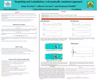
Developments of a dynamically consistent targeting and assimilation method

1. Developments of a dynamically consistent targeting and assimilation method Alberto Carrassi(°), Anna Trevisan(*) and Francesco Uboldi(§) (°) Dept. of Physics University of Ferrara, carrassi@fe.infn.it;(*)ISAC-CNR Bologna, A.Trevisan@isac.cnr.it; ( §)no affiliation, uboldi@magritte.it • Summary • A dynamically based assimilation method has recently been developed. • The basic idea is to exploit the flow dependent instabilities of the data assimilation cycle. The assimilation increment is confined within the unstable subspace where the most important components of the error are expected to grow. As a consequence the analysis update has the same structure as the estimated unstable structures. The analysis cycle is considered as an observationally forced dynamical system and the assimilation scheme itself is designed with the aim of stabilizing such a system. The unstable subspace is estimated by Breeding on Data Assimilation System (BDAS). • The theoretical basis of the proposed method and preliminary results in the context of a low-order nonlinear model were presented in a first work: • Trevisan, A. and F. Uboldi, 2004. Assimilation of Standard and Targeted Observations within the Unstable Subspace of the Observation-Analysis-Forecast Cycle System. J. Atmos. Sci., 61, 103-113. • Studies have been made to further investigate the development of the assimilation scheme and its applicability to more realistic environments. In the context of a quasi-geostrophic atmospheric model the performance of the method has been tested for the assimilation of adaptive observations. The ability of a data assimilation system to control the instabilities, responsible for error growth, can be improved by the combination of targeting strategies and a dynamically consistent assimilation. The benefit of adaptively located observations is greatly enhanced if their positions and their assimilation are designed in order to target the instabilities, estimated by BDAS. A comparison has been with a standard 3DVar assimilation scheme and the results have shown a dramatic reduction of the analysis error when the adaptive observations are assimilated using the proposed assimilation scheme. Moreover the reduction of the error is accompanied with a stabilization of the analysis cycle solution: the leading Lyapunov exponent which is positive in the free system and in the 3DVar assimilation cycle, becomes negative with our assimilation. Results of this application with an extended discussion of the approach is presented in: • Carrassi A., A. Trevisan and F. Uboldi, 2005. Deterministic Data Assimilation and Targeting by Breeding on the Data Assimilation System. In review for J. Atmos. Sci.. • The ability of the method to exploit a fixed observational network has been studied using a primitive-equation oceanic model. Here the proposed method has been compared with a standard Cooper-Haines assimilation scheme. Although less spectacular, a significant reduction of the error is obtained but when adaptive observations are added to the observational network and assimilated with the dynamically consistent method, the performance is greatly enhanced. The preliminary results of this application are described in: • Uboldi F., A. Trevisan and A. Carrassi, 2005. Developing a Dynamically Based Assimilation Method for Targeted and Standard Observations. Nonl. Pr. Geo., 12, 149-156 • Mathematical Formulation • The analysis increment is confined to the N-dimensional unstable subspace spanned by a set of N vectors en: • (1) • where xa is the analysis, xf is the forecast (background) state, E is the I x N matrix (I being the total number of degrees of freedom) whose columns are the envectors and the vector of coefficients a, the analysis increment in the unstable subspace, is the control variable . This is equivalent to estimating the forecast error covariance as: • (2) • where  represents the forecast error covariance matrix in the N-dimensional subspace spanned by the columns of E.The solution is : • (3) • here H is the (Jacobian of the) observation operator, R is the observation error covariance matrix, and yo is M-dimensional observation vector. It is intended here that N  M, so that for each vector en there is at least one observation. • For the theoretical discussion and detailed mathematical formulation see: [4] and [5]. • Outline of implementation • Estimate the unstable subspace is obtained by Breeding on the Data Assimilation System (BDAS); • Targetted observations are placed at locations where bred vectors en have maximum component; • A wide modulating function is used to isolate the regional structure of the bred vector; • A small number N of Bred Vectors are computed and used to construct the matrix E; • Use E to estimate Pfand confine the analysis increment in the unstable subspace: xa = xf+ Ea; • Conclusion • The main conclusion of this work is that the benefit of adaptive observations is greatly enhanced if their assimilation is based on the same dynamical principles as targetting. Results show that a few carefully selected and properly assimilated observations are sufficient to control the instabilities of the Data Assimilation System and obtain a drastic reduction of the analysis error. Further results (see [5]) obtained in the context of a primitive equation ocean model and regular observational network also proves the ability of the proposed assimilation method to reduce the error and efficiently exploit the estimated unstable subspace. The application of the method to a regular observational network and its extention to the four dimensional case are presently under study. The success obtained so far makes us very hopeful that, even in an operational environment with real adaptive observations, this method can yield significant improvement of the assimilation performance. References • [1]: detailed results and theoretical discussion: Carrassi A., A. Trevisan and F. Uboldi, 2005. Deterministic Data Assimilation and Targeting by Breeding on the Data Assimilation System. In review for J. Atmos. Sci.. • [2]: on the 3DVar scheme: Morss R., 1999. Adaptive Observations: Idealized sampling strategy for improving numerical weather prediction. PhD thesis, Massachussets of Technology, Cambridge, MA, 225 pp. • [3]: on the QG model: Rotunno R., and J. W. Bao, 1996. A case study of cyclogenesis using a model hierarchy. Mon. Wea. Rev., 124, 1051-1066 • [4]: a previous study with a small nonlinear model: Trevisan A., and F. Uboldi, 2004. Assimilation of standard and targeted observation within the unstable subspace of the observation-analysis-forecast cycle system. J. Atmos. Sci., 61, 103-113 • [5]: preliminary results of the oceanic application: Uboldi F., A. Trevisan and A. Carrassi, 2005. Developing a Dynamically Based Assimilation Method for Targeted and Standard Observations. Nonl. Pr. Geo., 12, 149-156 • APPLICATION TO A QG ATMOSPHERIC MODEL • The model is a 64x32 grid, 7 levels periodic channel [3]; the land area (longitudinal grid points 1-20) is completely covered by observations, assimilated by a 3DVAR scheme [2]. Adaptive observations are located over the ocean (longitudinal grid points 21-64) and are assimilated either with the proposed scheme, or, for comparison, with the same 3DVAR scheme used on land. • The unstable subspace of the data-forced system is estimated by means of BDAS, a modified breeding technique where all perturbed states undergo the same assimilation processes as the control state. A “regionalization” procedure is used to isolate maximum/minimum structures present in the forced bred vectors, and the analysis increment is confined in the subspace spanned by these structures. In this application only one unstable structure is used at each analysis time, and the adaptive observations are located at or around the maximum of the current structure, e. This vector is then used to assimilate the observations by means of equation (3). For a scalar observation yoeq. 3 reduces to: • where H is the linear observation operator. The last factor on the right-end side, used for a noisy observation, is estimated from the average over an appropriate time interval of the innovation, and it is equal to 1 when the observation is perfect. For further details and results, see [1]. • Comparison between two different experiments: • Experiment type I: all observations, fixed and adaptive, are assimilated by means of 3DVAR. The adaptive observation over the ocean is a vertical sounding of temperature and velocity components. • Experiment type II: the fixed observations are assimilated by means of 3DVAR; the adaptive observations by means of the proposed method. The adaptive obsrvations consist of 1 temperature obs. (exp. II-P and II-N); 1 temperature obs. and 1 velocity components at the same grid point (exp. II-P-2 and II-N-2); 5 temperature obs. (exp. II-P-5 and II-N-5) The adaptive observation in all experiments is placed at the location where the current bred vector attains its maximum amplitude FIG (1): Perfect observations. Normalized RMS analysis error as a function of time. The error is expressed in potential enstrophy norm and it is normalized by natural variability. Upper panel: Experiment I-P (3DVAR), adapt. obs. is a sounding; Middle panel: Experiment II-P, adapt. obs. is one temperature value; Lower panel: Experiment II-P-2, adpt. obs. is temperature and meridional velocity at same targeted grid point. FIG (2): Noisy observations. Same as fig (1) but using observations affected by error. Upper panel: Experiment I-N; Middle panel: Experiment II-N Lower Panel: Experiment II-N-5, adapt. obs. are 5 temperature values at grid points surrounding the targeted location. FIG (4): Forecast error as a function of the forecast range. Error is expressed in potential enstrophy norm and it is normalized by natural variability. Top panel: perfect obs. Lower panel: noisy obs., Dashed-dotted line: exp. I (3DVar). Continuous line: exp. II (proposed method-1 adapt. obs.). FIG (3): Background error (color) at two randomly chosen instants and analysis increment (black contour). Upper panel: exp. I-P (3DVAR); Lower panel: exp. II-P and Gaussian masking function (red contour). The area shown is a portion of the whole domain; note also that the interval between isolines of the analysis increment is different in the two panels. FIG (5): Leading Lyapunov exponent of the assimilation systems as a function of time (perfect observations). Values are averaged over all previous instants. The growth rate is expressed in units of days-1. Dotted line: Experiment I-P (3DVar); Continuous Line: Experiment II-P. PRIMITIVE EQUATION ISOPYCNAL OCEAN MODEL “MICOM” The configuration is a rectangular box with 180x140, 20km grid and 4 isopycnal layers (0-5000m). Perfect model, perfect observations. BDAS is implemented here with 36 perturbed trajectories, and the unstable structures are extracted from sets of 6 bred vectors at a time. A description of how the unstable structures are estimated and how they are used with the “standard observation” SSH field can be found in [5]. The panel on the right shows the sequence of forecast and analysis total energy errors, normalized with natural variability. RED: standard Cooper-Haines assimilation of “satellite” Sea Surface Height every 10 days. GREEN: the observed SSH field is used for eliminating the forecast error component on the estimated unstable subspace at standard analysis times. BLUE: 3 adaptive observations are added on days +2.5, +5.0, +7.5 after each SSH analysis, and assimilated with the proposed method. Complete results with standard and adaptive observations with this ocean system will be included in a manuscript in preparation.