Download
1 / 15
150 likes | 296 Views
Confidence Intervals for Capture-Recapture Data With Matching. Stephen Sharp, National Records of Scotland. The Problem (i). You have undertaken a (presumably imperfect) enumeration of a given population. You then undertaken a second (also presumably imperfect) coverage survey .

E N D
Confidence Intervals for Capture-Recapture Data With Matching Stephen Sharp, National Records of Scotland
The Problem (i) • You have undertaken a (presumably imperfect) enumeration of a given population. • You then undertaken a second (also presumably imperfect) coverage survey. • You have matched the two so that you know how many people were in both surveys (N12); in the first survey only (N1); and in the second survey only (N2). • You require to estimate the number of people in neither survey (N0).
The Problem (ii) • The classical estimate of N0 is the product of N1 and N2 divided by N12. • However this assumes that absence from the first survey does not change the probability of absence from the second. • For humans, this is very unlikely.
A Bayesian approach • As we do not know N0, we require its probability distribution conditional on N12, N1 and N2 which we do know. • We get this from Bayes’ theorem. • p(N0 | N12 N1 N2) = constant x p(N12 N1 N2 | N0) x p(N0). • Posterior is proportional to likelihood x prior. • We need a likelihood and a prior.
The likelihood function (i) • The distribution of N12, N1 and N2 conditional on N0 is multinomial with probability parameters p12, p1, p2 and p0. • The four probabilities must sum to one so we need three constraints to specify uniquely three parameters. • We assume that p12, p1 and p2 stand in the same proportions as N12, N1 and N2. • This gives us two constraints.
The likelihood function (ii) • Instead of imposing a third constraint however we let the posterior distribution of N0 depend on the dichotomous correlation ϕ, which measures stochastic dependency. • We can now specify the likelihood for a given value of ϕ and watch the effect of changing it.
The prior distribution • What did we know about the likely size of the population before we took the two surveys? • This knowledge is reflected in the prior distribution. • A safe bet would be an uninformative prior (perhaps a normal or uniform distribution with a very big variance). • If you are confident though you might be better to use an informative prior (i.e. a smaller prior variance). • This reduces the variance of the posterior distribution (though be careful to check that the prior is consistent with the likelihood).
Further work (i) • So we can model the point estimate and confidence intervals as a function of the dichotomous correlation f. • But what is the value of f? • This will vary from one subgroup to another within the population. • It will depend on the diversity within the subgroup of the propensity to take part in public surveys like the Census and the coverage survey.
Further work (ii) • Attempts to model this have suggested that typical values for f vary between 0.25 and 0.40. • This suggests that for an uninformative prior, the population point estimate might be 560 against 520 with the independence assumption; an underestimate of about 7%. • The confidence intervals are ±14 or 15 as opposed to ±6 or 7; about twice as wide.
Conclusion • The assumption of independence introduces error into both the point estimate and the confidence intervals when population size is estimated from capture-recapture data. • The CI error is in the “wrong” direction (i.e. not on the side of caution). • Departure from independence arises because those members of the population unlikely to be included in one sample are less likely to be included in the other. • Assessing the extent of dependence is difficult but its effects make it important to try.
Confidence Intervals for Capture-Recapture Data With Matching Stephen Sharp National Records of Scotland Ladywell House Ladywell Road Edinburgh EH12 7TF 0131 314 4649 Stephen.sharp@gro-scotland.gsi.gov.uk