Download
1 / 18
220 likes | 1.65k Views
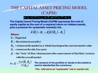
Capital Asset Pricing Model (CAPM). Assumptions Investors are price takers and have homogeneous expectations One period model Presence of a riskless asset No taxes, transaction costs, regulations or short-selling restrictions (perfect market assumption)

E N D
Capital Asset Pricing Model (CAPM) Assumptions • Investors are price takers and have homogeneous expectations • One period model • Presence of a riskless asset • No taxes, transaction costs, regulations or short-selling restrictions (perfect market assumption) • Returns are normally distributed or investor’s utility is a quadratic function in returns
CAPM Derivation Return Efficientfrontier m rf Sp A. For a well-diversified portfolio, the equilibrium return is: E(rp) = rf + [E(rm-rf)/sm]sp
For the individual security, the return-risk relationship is determined by using the following (trick):rp = wri + (1-w)rmsp=[w2s2i +(1-w)2s2m+2w(1-w)sim]0.5where sim is the covariance of asset iand market (m) portfolio, and w is the weight. drp/dw = ri -rm 2ws2i -2(1-w)s2m+2sim-4wsim 2sp dsp/dw =
w=0 ri -rm (sim-s2m)/sm sim - s2m = sm drp/dw = dsp/dw • dsp/dw w=0 The slope of this tangential portfolio at M must equal to: [E(rm) -rf]/sm,Thus, ri -rm = [rm-rf]/sm (sim-s2m)/sm Thus, we have CAPM as ri = rf + (rm-rf)sim/s2m
Properties of SLM If we express the return-risk relationship as beta, then we haveri = rf + E(rm -rf) bi Return SML E(rm ) rf beta=1 RISK
Return q p z covip -covpq E(ri) = E(rq) + [E(rp)-E(rq)] s2p -covpq Zero-beta CAPM • No Riskless Asset s2p where p, q are any two arbitrary portfolios
CAPM and Liquidity • If there are bid-ask spread (c) in trading asset i, then we have: • E(ri) = rf + bi[E(rm)-rf] + f(ci)where f is a non-linear function in c (trading cost).
Single-index Model • Understanding of single-index model sheds light on APT (Arbitrage Pricing Theory or multiple factor model) • suppose your analyze 50 stocks, implying that you need inputs:n =50 estimates of returnsn =50 estimates of variancesn(n-1)/2 = 50(49)/2=1225 (covariance) • problem - too many inputs
Factor model(Single-index Model) • We can summarize firm return, ri, is:ri = E(ri)+mi + eiwhere mi is the unexpected macro factor; ei is the firm-specific factor. • Then, we have:ri = E(ri) + biF + eiwhere biF = mi, and E(mi)=0 • CAPM implies:E(ri) = rf + bi(Erm-rf) in ex post form,ri =rf + bi(rm-rf) + eiri = [rf+bi(Erm-rf)]+bi(rm-Erm) + ei ri = a + bRm + ei
Total variance: s2i = b2is2m + s2(ei)The covariance between any two stocks requires only the market index because ei and ej is assumed to be uncorrelated. Covariance of two stocks is: cov(ri, rj) =bibjs2mThese calculations imply: n estimates of return n estimates of beta n estimates of s2(ei) 1 estimate of s2mIn total =3n+1 estimates required Price paid= idiosyncratic risk is assumed to be uncorrelated
Index Model and Diversification • ri = a + biRm +ei • rp=ap +bpRm +eps2p=b2ps2m + s2(ep)where:s2(ep) = [s2(e1)+...s2(en)]/n(by assumption only! Ignore covariance terms)
Market Model and Empirical Test Form • Index (Market) Model for asset i is: • ri = a + biRm + ei Excess return, i slope=beta =cov(i,m)s2m Rm R2 =coefficient of determination = b2s2m/s2i
Arbitrage Pricing Theory (APT) • APT - Ross (1976) assumes:ri =E(ri) + bi1Fi+...+bikFk + eiwhere:bik =sensitivity of asset i to factor kFi = factor and E(Fi)=0 • Derivation:w1+...+wn=0 (1)rp =w1r1+...wnrn =0 (2) • If large no. of securities (1/n tends to 0), we have:Systematic + unsystematic risk=0(sum of wibi) (sum of wiei)
That means: w1E(r1)+...wnE(rn) =0 (no arbitrage condition) Restating the above conditions, we have:w1 + ...wn =0 (0)w1b1k +...+wnbnk=0 for all k (1) Multiply:d0 to w1+...wn =0 (0’) d1 to w1d1b11+...wnd1bn1=0 (1-1) dk to w1dkb1k+...wndkbnk=0 (1-k) Grouping terms vertically yields: w1(d0+d1b11+d2b12+...dkb1k)+w2(d0+d1b21+d2b22+...dkb2k )+wn(d0+d1bn1+d2bn2+...dkbnk)=0 E(ri) = d0 + d1bi1+...+dkbik (APT)
If riskless asset exists, we have rf =d0, which then implies: APT: E(ri) -rf = d1bi1 + ...+dkbik , and di = risk premium =Di -rf
APT is much robust than CAPM for several reasons: 1. APT makes no assumptions about the empirical distribution of asset returns; 2. APT makes no assumptions on investors’ utility function; 3. No special role about market portfolio 4. APT can be extended to multiperiod model.
Illustration of APT • Given: • Asset Return Two Factors bi1 bi2 x 0.110.5 2.0 y 0.25 1.0 1.5 z 0.23 1.5 1.0 • D1=0.2; D2=0.08 and rf=0.1 E(ri)=rf + (Di-rf)bi1+ (D2-rf)bi2 E(rx)=0.1+(0.2-0.1)0.5+(8%-0.1)2=11% E(ry)=0.1+(0.2-0.1)1+(8%-0.1)1.5=17% E(rz)=0.1+(0.2-0.1)1.5+(8%-0.1)1=23%
Suppose equal weights in x,y and z i.e., 1/3 each Risk factor 1=(0.5+1.0+1.5)/3=1 Risk factor 2=(2+1.5+1.)/3 =1.5 Assume wx=0;wy=1;wz=0Risk factor 1= 1(1.0)=1 Risk factor 2= 1(1.5)=1.5 Original rp=(0.11+0.25+0.23)/3=19.67% New rp=0(11%)+1(25%)+0(23%)=25%