Download
1 / 41
450 likes | 732 Views
ACTIVE FILTER CIRCUITS. DISADVANTAGES OF PASSIVE FILTER CIRCUITS. Passive filter circuits consisting of resistors, inductors, and capacitors are incapable of amplification, because the output magnitude does not exceed the input magnitude.

E N D
DISADVANTAGES OF PASSIVE FILTER CIRCUITS • Passive filter circuits consisting of resistors, inductors, and capacitors are incapable of amplification, because the output magnitude does not exceed the input magnitude. • The cutoff frequency and the passband magnitude of passive filters are altered with the addition of a resistive load at the output of the filter. • In this section, filters using op amps will be examined. These op amp circuits overcome the disadvantages of passive filter circuits.
C R2 R1 + + + vi + vo FIRST-ORDER LOW-PASS FILTER Zf Zi + vi + vo
PROTOTYPE LOW-PASS FIRST-ORDER OP AMP FILTER Design a low-pass first-order filter with R1=1Ω, having a passband gain of 1 and a cutoff frequency of 1 rad/s.
FIRST-ORDER HIGH-PASS FILTER R2 C R1 + vi + vo + Prototype high-pass filter with R1=R2=1Ω and C=1F. The cutoff frequency is 1 rad/s. The magnitude at the passband is 1.
EXAMPLE Figure shows the Bode magnitude plot of a high-pass filter. Using the active high-pass filter circuit, determine values of R1 and R2. Use a 0.1μF capacitor. If a 10 KΩ load resistor is added to the filter, how will the magnitude response change?
Notice that the gain in the passband is 20dB, therefore, K=10. Also note the the 3 dB point is 500 Hz. Then, the transfer function for the high-pass filter is Because the op amp in the circuit is ideal, the addition of any load resistor has no effect on the behavior of the op amp. Thus, the magnitude response of the high-pass filter will remain the same when a load resistor is connected.
SCALING In the design of both passive and active filters, working with element values such as 1 Ω, 1 H, and 1 F is convenient. After making computations using convenient values of R, L, and C, the designer can transform the circuit to a realistic one using the process known as scaling. There are two types of scaling: magnitude and frequency. A circuit is scaled in magnitude by multiplying the impedance at a given frequency by the scale factor km. Thus, the scaled values of resistor, inductor, and capacitor become where the primed values are the scaled ones.
In frequency scaling, we change the circuit parameter so that at the new frequency, the impedance of each element is the same as it was at the original frequency. Let kf denote the frequency scale factor, then A circuit can be scaled simultaneously in both magnitude and frequency. The scaled values in terms of the original values are
EXAMPLE This circuit has a center frequency of 1 rad/s, a bandwidth of 1 rad/s, and a quality factor of 1. Use scaling to compute the values of R and L that yield a circuit with the same quality factor but with a center frequency of 500 Hz. Use a 2 μF capacitor. 1H 1F + vi + vo 1Ω The frequency scaling factor is: The magnitude scaling factor is:
EXAMPLE Use the prototype low-pass op amp filter and scaling to compute the resistor values for a low-pass filter with a gain of 5, a cutoff frequency of 1000 Hz, and a feedback capacitor of 0.01 μF. To meet the gain specification, we can adjust one of the resistor values. But, changing the value of R2 will change the cutoff frequency. Therefore, we can adjust the value of R1 as R1=R2/5=3183.1 Ω.
OP AMP BANDPASS FILTERS • A bandpass filter consists of three separate components • A unity-gain low-pass filter whose cutoff frequency is wc2, the larger of the two cutoff frequencies • A unity-gain high-pass filter whose cutoff frequency is wc1, the smaller of the two cutoff frequencies • A gain component to provide the desired level of gain in the passband. • These three components are cascaded in series. The resulting filter is called a broadband bandpass filter, because the band of frequencies passed is wide.
CL RH Rf RL RL CH RH Ri + + + + vi + vo Vo Vi Low-pass filter High-pass filter Inverting amplifier
Standard form for the transfer function of a bandpass filter is In order to convert H(s) into the standard form, it is required that . If this condition holds, Then the transfer function for the bandpass filter becomes
Compute the values of RL and CL to give us the desired cutoff frequency Compute the values of RH and CH to give us the desired cutoff frequency To compute the values of Ri and Rf, consider the magnitude of the transfer function at the center frequency wo
EXAMPLE Design a bandpass filter to provide an amplification of 2 within the band of frequencies between 100 and 10000 Hz. Use 0.2 μF capacitors. Arbitrarily select Ri=1 kΩ, then Rf=2Ri=2 KΩ
OP AMP BANDREJECT FILTERS • Like the bandpass filters, the bandreject filter consists of three separate components • The unity-gain low-pass filter has a cutoff frequency of wc1, which is the smaller of the two cutoff frequencies. • The unity-gain high-pass filter has a cutoff frequency of wc2, which is the larger of the two cutoff frequencies. • The gain component provides the desired level of gain in the passbands. • The most important difference is that these components are connected in parallel and using a summing amplifier.
+ + + CL RL RL Ri Rf + Ri vo vi + RH CH RH
The magnitude of the transfer function at the center frequency
HIGHER ORDER OP AMP FILTERS All of the filters considered so far are nonideal and have a slow transition between the stopband and passband. To obtain a sharper transition, we may connect identical filters in cascade. For example connecting two first-order low-pass identical filters in cascade will result in -40 dB/decade slope in the transition region. Three filters will give -60 dB/decade slope, and four filters should have -80 db/decade slope. For a cascaded of n protoptype low-pass filters, the transfer function is
But, there is a problem with this approach. As the order of the low-pass is increased, the cutoff frequency changes. As long as we are able to calculate the cutoff frequency of the higher-order filters, we can use frequency scaling to calculate the component values that move the cutoff frequency to its specified location. For an nth-order low-pass filter with n prototype low-pass filters
EXAMPLE Design a fourth-order low-pass filter with a cutoff frequency of 500 rad/s and a passband gain of 10. Use 1 μF capacitors. Thus, R=138.46Ω and C=1 μF. To set the passband gain to 10, choose Rf/Ri=10. For example Rf=1384.6 Ω and Ri =138.46 Ω.
+ + + + + 1μF 1μF 1μF 138.46Ω 138.46Ω 138.46Ω 138.46Ω 138.46Ω 138.46Ω vi + 1μF 1384.6Ω 138.46Ω 138.46Ω 138.46Ω + vo
By cascading identical prototype filters, we can increase the asymptotic slope in the transition and control the location of the cutoff frequency. But the gain of the filter is not constant between zero and the cutoff frequency. Now, consider the magnitude of the transfer function for a unity-gain low-pass nth order cascade.
BUTTERWORTH FILTERS A unity-gain Butterworth low-pass filter has a transfer function whose magnitude is given by • The cutoff frequency is wc for all values of n. • If n is large enough, the denominator is always close to unity when w<wc. • In the expression for |H(jw)|, the exponent of w/wc is always even.
Given an equation for the magnitude of the transfer function, how do we find H(s)? To find H(s), note that if N is a complex quantity, the |N|2=NN*. Then,
The procedure for finding H(s) for a given n is: • Find the roots of the polynomial 1+(-1)ns2n=0 • Assign the left-half plane roots to H(s) and the right-half plane roots to H(-s) • Combine terms in the denominator of H(s) to form first- and second-order factors
EXAMPLE Find the Butterworth transfer function for n=2. For n=2, 1+(-1)2s4=0, then s4=-1=1 1800 Roots s2 and s3 are in the left-half plane. Thus,
BUTTERWORTH FILTER CIRCUITS To construct a Butterworth filter circuit, we cascade first- and second-order op amp circuits using the polynomials given in the table. A fifth-order prototype Butterworth filter is shown in the following figure: vi vo All odd-order Butterworth polynomials include the factor (s+1), so all odd-order BUtterworth filters must include a subcircuit to implement this term. Then we need to find a circuit that provides a transfer function of the form
+ C1 R R + Va Vo + C2 vi
EXAMPLE Design a fourth-order low-pass filter with a cutoff frequency of 500 Hz and a passband gain of 10. Use as many 1 KΩ resistor as possible. From table, the fourth-order Butterworth polynomial is For the first stage: C1=2/0.765=2.61 F, C2=1/2.61=0.38F For the second stage: C3=2/1.848=1.08 F, C4=1/1.08=0.924F These values along with 1-Ω resistors will yield a fourth-order Butterworth filter with a cutoff frequency of 1 rad/s.
+ + + A frequency scale factor of kf=3141.6 will move the cutoff frequency to 500 Hz. A magnitude scale factor km=1000 will permit the use of 1 kΩ resistors. Then, R=1 kΩ, C1=831 nF, C2=121 nF, C3= 344 nF, C4=294 nF, Rf= 10 kΩ. Rf C3 C1 Ri R R R R + Vo C4 + C2 vi
The Order of a Butterworth Filter As the order of the Butterworth filter increases, the magnitude characteristic comes closer to that of an ideal low-pass filter. Therefore, it is important to determine the smallest value of n that will meet the filtering specifications. |H(jw)| Transition band Stop band Pass band WP WS log10w AP AS
If wp is the cutoff frequency, then For a steep transition region, Thus,
EXAMPLE Determine the order of a Butterworth filter that has a cutoff frequency of 1000 Hz and a gain of no more than -50 dB at 6000 Hz. What is the actual gain in dB at 6000 Hz? Because the cutoff frequency is given, and 10-0.1(-50)>>1 Therefore, we need a fourth-order Butterworth filter. The actual gain at 6000 Hz is
EXAMPLE Determine the order of a Butterworth filter whose magnitude is 10 dB less than the passband magnitude at 500 Hz and at least 60 dB less than the passband magnitude at 5000 Hz. Thus we need a third-order filter. Determine the cutoff frequency.
+ BUTTERWORTH HIGH-PASS FILTERS To produce the second-order factors in the Butterworth polynomial, we need a circuit with a transfer function of Setting C= 1F R1 C C + Vo + R2 vi
NARROWBAND BANDPASS AND BANDREJECT FILTERS The cascade or parallel component designs from simpler low-pass and high-pass filters will result in low-Q filters. Consider the transfer function Thus with discrete real poles, the highest quality factor bandpass filter we can achieve has Q=1/2