Download
1 / 22
220 likes | 423 Views
Statistical techniques have underlying assumptions.Graphs aid in the checking of a list of underlying assumptions.All statistical techniques require assumptions.For example, regression analysis requires the model residuals are randomly distributed.Residual plots must show random scatter rather t

E N D
1. Graphs Introduction
Ecological Fallacy
Opening, Importing, Creating Data
Data Summaries
Single-Variable Graphs
Scatterplots
2. Statistical techniques have underlying assumptions.
Graphs aid in the checking of a list of underlying assumptions.
All statistical techniques require assumptions.
For example, regression analysis requires the model residuals are randomly distributed.
Residual plots must show random scatter rather than a systematic pattern. If not your interpretation of results will be misleading.
Graphs are the heart of most statistical analysis; corresponding tables are formal confirmations of our visual impressions.
Graphs are not automatically produced by the software.
The analyst must request them.
A graph is a geometrical representation of information in a table of numbers.
The goal of statistical graphics is to make evident the characteristics of the data such as location, variability, scale, shape, correlation, interaction, and clustering.
Once we have a visual understanding of the data, we attempt to model it with formal algebraic procedures.
In this class we will work with lots of data, either
Imported from outside of Splus, or
Intrinsic to Splus.
3. Ecological Fallacy Examining plots early on in the data analysis procedure is essential.
The point is demonstrated by what is known as the ecological fallacy.
If without examining a plot of these (simulated) data we perform a simple regression of y on x, we find that y and x are directly related.
However, the plot strongly suggests that we have an amalgamation of 3 separate groups.
Within each of the groups it is clear that y and x are inversely related.
Robinson (1950) coined the terms ecological fallacy and ecological correlation.
He noted that the correlation between percentage illiterate and percentage black racial group for the US as a whole (1930 Census) is different from this correlation within various subgroups of the US population.
Human ecology is a branch of sociology dealing with the relationship between human groups and their environments.
4. To open an intrinsic data set click Data > Select Data.
Type in lynx under Name then click OK.
Then select Open read-only.
The data are annual number of lynx trappings in the Mackenzie River District of Northwest Canada for the period 1821-1934.
Click on the gray area in the top of the column labeled Data to highlight it. The entire column gets highlighted in black.
The word double indicates that the data values are in double precision, which means the arithmetic gets performed on 64 bits instead of 32 bits.
To highlight a row, click on the gray area to left of the row.
Splus has several intrinsic data sets that are of interest to us.
The data sets are not fabricated.
Other data sets will be provided online either in ASCII text or Excel format.
6. Download Duncan.txt from Blackboard under Course Library > Datasets.
Right click and Save Target As.
Save to Desktop.
Import a data set from your Desktop click File > Import Data > From File.
Browse to your desktop and select Duncan.txt then click OK.
Change File Format to ASCII file � comma delimited (csv) then click OK.
Note: At the bottom of all Splus dialog boxes is a recall button.
This allows you to recall what you input previously.
This helps when you make an error and when you repeat tasks.
7. The data in the Data object Duncan were originally analyzed by Duncan (1961).
The first row provides the column names (job, income, education, prestige). Hold the cursor above the column to see that the data type is factor.
Each subsequent row contain data. Rows are numbered.
The variables are:
job : Title (factor)
income : Percentage of occupational incumbents in the 1950 US Census who earned more than $35K/yr.
education : Percentage who where high-school graduates.
prestige : Percentage of respondents in a social survey who rated their occupation as good or better in prestige.
Duncan performed a regression of prestige on income and education. His interest was to predict the prestige levels of occupations for which income and educational levels where known, but for which there were no direct prestige ratings.
Splus can import data from a variety of formats.
Often data are imported from MS Excel files with extension .xls.
If the Excel file contains multiple sheets, each sheet must be individually imported by saving a new Excel file with the sheet in the first position and then importing the new file.
9. Use the attach command from the Command Window to allow access to its columns.
> attach(Duncan)
> prestige
This gives us access to the data in the columns without invoking the name of the data set.
To find the mean prestige ranking, type
> mean(prestige)
[1] 47.48889
> median(education)
[1] 45
> stdev(income)
[1] NA
> stdev(income,na=T)
[1] 24.28418
> range(education)
[1] 7 100
Data Summaries
11. Although the summary function gives you some idea of the shape of the data, you can do better with graphs.
A good graphical display of information can eliminate the need for further statistical analysis.
On the other hand, all graphs are subject to over-interpretation�in particular, you can be fooled by randomness.
Several principles should be followed when graphing data.
Choose a display that is understandable.
Pleasing to the eye and not too simple or overly complicated.
Faithfully represent the data.
When grouping and summarizing data some information is inevitably lost. Convey as much information as possible.
Some displays hide an aspect of the data.
This should be made clear to the viewer in the display or in a footnote to the display.
Using the GUI in Splus, plots are constructed using the Plots 2D palette. Single-Variable Graphs
12. Boxplot: The boxplot is a visual display based on 5 summary values (minimum, maximum, median, 1st and 3rd quartiles).
Close the Duncan data sheet.
Reopen the lynx.df data frame by double clicking on the shortcut in the Object Explorer.
Click on the top of the Data column to darken it.
Click on the Box icon on the Plots 2D palette.
The result is a standard box plot.
The median value is denoted by the thin red line inside the box with a dot on it.
The 1st (lower) quartile is denoted by the bottom of the box and the 3rd (upper) quartile is denoted by the top of the box.
The interquartile distance (IQD) is 3rd quartile value minus 1st quartile value.
If there are values that exceed 1.5 times the IQD from the mean value in either direction (above or below), they are plotted as lines with dots on them.
Otherwise the minimum or maximum value is displayed.
13. General information.
Graphs are created in and can be saved as Graph Sheets.
Saved Graph Sheets have the file extension .sgr, which can be opened later even after you have quit and restarted Splus.
Multiple plots can be combined on one graph, multiple graphs can be combined on one Graph Sheet, and Graph Sheets can contain multiple pages.
Graph Sheets can be exported to image formats such as JPG, GIF, and TIF.
There are 3 areas of the graph sheet.
The Graph Sheet is the actual page the plot is drawn on.
Attributes such as the margin, orientation, and spacing are specified in the Graph Sheet Properties dialog.
The graph area is outside the plot axis, but within the Graph Sheet.
The plot area is the area of the plot including the axes.
The plot is the actual points of the graph.
15. The standard boxplot shows 4 outliers at the high range.
These values are greater than 1.5 times the IQD from the mean.
Note there are no outliers below the mean value. This is an indication of positively skewed data.
Left click in the box area of the box plot, then double click to open the Box Plot dialog box.
Select the Box Specs tab and change Whisker Style from Standard to Simple.
Change the axis label.
Resize the plot making it narrower.
16. Histogram: A histogram is a graph showing the distribution of data values.
It divides the range of data values into non-overlapping intervals (bins).
The number of values which fall into each interval is counted.
Bars are plotted with height proportional to the count.
It is the most common graph for examining a sample distribution of a quantitative variable.
Single click on the Data column in the lynx.df to darken it.
Select the Histogram button the Plots 2D palette.
Click anywhere inside the plot (blue shaded histogram), then double click on the green square to open the Histogram/Density dialog box.
Under the Options tab, type 0 for Lower Bound and type 8000 for Upper Bound.
Type 16 in the Number of Bars field, then OK.
Change the x-axis label appropriately.
17. Density plot: A density plot is a smooth version of a histogram.
They provide estimates of the underlying population frequency.
Close the lynx.df.
Click Data > Select Data, in the dialog box type air in the Name field.
The data are taken from an environmental study that measured 4 variables of ozone (ppm), solar radiation, air temperature (F), and wind speed (mph) for 111 consecutive days (Chambers and Hastie 1992).
Highlight the ozone column.
On the Plots 2D palette, click on Density.
Add a title and proper axes labels.
Since the density curve is smooth, it is more pleasant to look at than the histogram.
The ozone data appear to come from a normal distribution.
A similar plot can be made in using the Command Window.
> densityplot(~air$ozone)
Here the density plot includes the a plot of the actual values above the horizontal axis.
The density curve is higher where points cluster.
The central clustering is around a value of 3 or so, but there is another clustering around 4.2.
18. Stem-and-leaf plot: A stem-and-leaf plot is a graph that shows groups of data arranged by place value.
The shape of the stem-and-leaf plot looks like a histogram.
Example: Consider the number of sit-ups a group of 13 students did in one minute.
stem : leaves
3 : 4 6 8 8
4 : 0 3 6 6 7
5 : 0 0 1 2
key 3 : 6 = 36
The number of leaves equals the number of students. The leaves are displayed to the right of the stem.
For the ozone data, type
> stem(air$ozone)
19. QQ plot: A quantile is a specific data value that divides the distribution of all data values into two parts, those values greater than the quantile value and those values less than the quantile value.
For instance, p percent of the values are less than the pth quantile.
Quantiles that divide the distribution into quarters (thirds) are called quartiles (terciles).
Quantiles that divide the distribution into tenths (fifths) are called deciles (quintiles).
A quantile-quantile (qq) plot is a two-dimensional graph of the ordered quantile values of one variable plotted against the ordered quantile values of another variable.
A normal qq plot uses the quantiles of the standard normal distribution as one of the variables and the quantiles of your data as the other variable.
The standard normal distribution has a mean of 0 and a standard deviation of 1.
If the normal qq plot is reasonably linear, then your data are approximately normally distributed.
Using the air data set, highlight the ozone column, then select the QQ Normal icon on the Plots 2D palette.
20. The normal qq plot is one of several plots used to compare distributions of data in hand with specified distributions.
It can also be used to compare distributions of two variables.
If two distributions are the same, the points of the qq plot will fall on a straight line.
Of the plots, the histogram and density plot give the best overall picture of the distribution shape of your data.
The boxplot and the normal qq plot give the clearest display of outliers.
When presented with more than one variable, it is frequently necessary to consider relationships between the variables.
The scatterplot is the most useful of all statistical graphs.
It shows whether we should further explore the possibility of a relationship between two variables.
21. Scatterplot: A scatterplot is a graph in which data values are represented as dots in 2 dimensions.
In a simple scatterplot, values of one variable are arrayed along the vertical axis (y-axis or ordinate) while values from another variable are arrayed along the horizontal axis (x-axis or abscissa).
In the context of regression analysis, we choose to plot the chosen dependent variable along the vertical axis.
The plotting routine automatically determines the appropriate scale and tick locations for both axes and prints the variable names as the default labels for the axes.
Open the Duncan data object, click on income, then hold the control (Ctrl) key down and click on prestige (called control clicking) to highlight both columns.
The first column selected will be plotted on the abscissa.
On the Plots 2D palette select Scatter.
Change Aspect Ratio to Proportional Units.
Label axes appropriately.
22. Graphs can be examined and labeled in more detail.
For example, we see 2 outliers, but which jobs do they represent?
Move your mouse over the point and leave it. The graph will respond with a call-out box indicating the values for income and prestige along with the corresponding row number.
We can go back to the data file and see that this corresponds to Minister.
We can label this point on the graph by opening the Graph Tools palette and selecting Label Point.
Move the cross hair over the point on the plot you want labeled and click.
We can label all points by values in another column.
Left click on any point, then double click on the green square to open the Line/Scatter Plot dialog box.
Select the Symbol tab and fill in as shown to the right, then click OK.