Download
1 / 49
490 likes | 710 Views
Geometric Interpretation of Linear Programs. Chris Osborn, Alan Ray, Carl Bussema, and Chad Meiners 16 March 2005. Introduction. Visualizing algebraic concepts geometrically can give new insight and understanding Understand properties of LP in terms of geometry

E N D
Geometric Interpretation of Linear Programs Chris Osborn, Alan Ray, Carl Bussema, and Chad Meiners 16 March 2005
Introduction • Visualizing algebraic concepts geometrically can give new insight and understanding • Understand properties of LP in terms of geometry • Use geometry as aid to solve LP • Model geometric problems as LP • Some concepts from earlier chapters; some new
Overview • Feasibility • Simplex Method • Simplex Weaknesses • Exponential Iterations • Degeneracy • Graphic Method • Duality • Convex Sets and Hulls
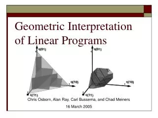
Region of Feasibility • Graphical region describing all feasible solutions to a linear programming problem • In 2-space: polygon, each edge a constraint • In 3-space: polyhedron, each face a constraint
Feasibility in 2-Space • 2x1 + x2≤ 4 • In an LP environment, restrict to Quadrant I since x1, x2≥ 0
Feasibility in 3-Space • Five total constraints; therefore 5 faces to the polyhedron
Simplex Method • Every time a new dictionary is generated: • Simplex moves from one vertex to another vertex along an edge of polyhedron • Analogous to increasing value of a non-basic variable until bounded by basic constraint • Each such point is a feasible solution
Simplex Illustrated: Initial Dictionary Current solution: x1 = 0 x2 = 0 x3 = 0
Simplex Illustrated: First Pivot Current solution: x1 = 0 x2 = 0 x3 = 5
Simplex Illustrated: Second Pivot Current solution: x1 = 2 x2 = 0 x3 = 5
Simplex Illustrated: Final Pivot Final solution (optimal): x1 = 0 x2 = 4 x3 = 5
Simplex Review and Analysis • Simplex pivoting represents traveling along polyhedron edges • Each vertex reached tightens one constraint (and if needed, loosens another) • May take a longer path to reach final vertex than needed
Cases with high complexity (2n-1 iterations) Normal complexity is O(m3) How was this problem solved? Simplex Weaknesses: Exponential Iterations: Klee-Minty Reviewed
Geometric Interpretation & Klee-Minty • Saw non-optimal solution earlier • How can we represent the Klee-Minty problem class graphically?
Step 1: Constructing a Shape • Start with a cube. • What characteristics do we want the cube to have? • What is the worst case to maximize z?
Step 1: Constructing a Shape • Goal 1: Create a shape with a long series of increasing facets • Goal 2: Create an LP problem that forces this route to be taken
[0, 1, 0.8] [0, 1, 0.82] [1, 0, 0.98] [0, 0, 1] [1, 0.8, 0] [0, 1, 0] [1, 0, 0] [0, 0, 0] Step 2: Increasing Objective Function: Modifying the Cube • Squash the cube • New dictionary
Step 3: Achieving 2n-1 Iterations: Altering the Algebra Let Convert to
The Final Solution • Most desirable: • Least desirable:
Simplex Weaknesses:Degeneration: Summary • How does the degeneracy of this problem impact the graphical solution? • Degenerate solutions express the same vertex in a different way. • How have we dealt with degeneracy previously?
Different Facets, One Point • We shift the multiple facets into two, separate ones [0, 0, 1] [0, 0, 1+0.25e2] [e - e2, 0, 1 + 0.25e2]
Non-Graphic Example • Where is the fourth colliding facet in this example: • Sometimes, degeneracy occurs without visible fourth facets (as above)
The Graphic Method • Use geometry to quickly solve LP problems in 2 variables • Plot all restrictions in 2D plane (x1, x2) • Result plus axes forms polyhedron • Region of feasible solutions • Draw any line with same slope as objective function through polyhedron • “Move” line until leaving feasible region • i.e., Find parallel tangent
Graphic Method Example:Step 1: Plot Boundary Conditions max 5x1 + 4x2 subject to: x1 – 3x2 ≤ 3 2x1 + 3x2 ≤ 12 -2x1 + 7x2 ≤ 21 x1,x2 ≥ 0
Graphic Method Example:Step 2: Determine Feasibility max 5x1 + 4x2 subject to: x1 – 3x2 ≤ 3 2x1 + 3x2 ≤ 12 -2x1 + 7x2 ≤ 21 x1,x2 ≥ 0 Based only on this, where might the optimal solution be?
Graphic Method Example:Step 3: Plot Objective = c max 5x1 + 4x2 subject to: x1 – 3x2 ≤ 3 2x1 + 3x2 ≤ 12 -2x1 + 7x2 ≤ 21 x1,x2 ≥ 0
Graphic Method Example:Step 4: Find Parallel Tangent max 5x1 + 4x2 subject to: x1 – 3x2 ≤ 3 2x1 + 3x2 ≤ 12 -2x1 + 7x2 ≤ 21 x1,x2 ≥ 0 Optimal solution: x1=5, x2=2/3, z=83/3
Graphic Method Discussion • Pro: • Works for any number of constraints • Fast, especially with graphing tool • Gives visual representation of tradeoff between variables • Con: • Only works well in 2D (feasible but difficult in 3D) • For very large number of constraints, could be annoying to plot • For large range / ratio of coefficients, plot size limits precision and ability to quickly find tangent
Second Graphic Method Example max 4x1 + 6x2 subject to: x1 – 3x2 ≤ 3 2x1 + 3x2 ≤ 12 -2x1 + 7x2 ≤ 21 x1,x2 ≥ 0 Same constraints; new objective. What changes?
Second Graphic Method Example:No Tangent Exists max 4x1 + 6x2 subject to: x1 – 3x2 ≤ 3 2x1 + 3x2 ≤ 12 -2x1 + 7x2 ≤ 21 x1,x2 ≥ 0 Optimal solution: 1.05 ≤ x1 ≤ 5, 2x1 + 3x2 = 12, z=24
Consider earlier problem:max 5x1 + 4x2 subject to: x1 – 3x2 ≤ 3 2x1 + 3x2 ≤ 12 -2x1 + 7x2 ≤ 21 x1,x2 ≥ 0 Optimal: x1*=5, x2*=2/3 Prove optimal if equal to corresponding dual solution min 3y1 + 12y2 + 21y3 subject to: y1 + 2y2 – 2y3 ≥ 5 -3y1 + 3y2 + 7y3 ≥ 4 y1, y2 ≥ 0 Geometric Interpretation of Duality
Geometric Duality Continued • Think of dual variables as coefficients for primal constraints (α = y1, = y2, = y3):(α) (x1 – 3x2) ≤ (α) 3() (2x1 + 3x2) ≤ () 12() (-2x1 + 7x2) ≤ () 21 • Resulting sum is linear combination:(α+2-2)x1 + (-3α+3+7)x2 ≤ 3α+12+21 • We can graph this for various choices of α, , and
Geometric Duality: Linear Combinations Graphed (α+2-2)x1 + (-3α+3+7)x2 ≤ 3α+12+21 • Three examples shown • α = = 1, = 0 • α = = = 1 • α = 0, = = 1 • Pink line is parallel tangent • Notice: primal solution two vertices away from origin • Two constraints matter; third irrelevant here. • Duality implication: = 0
Geometric Duality Graphed Again (α+2)x1 + (-3α+3)x2 ≤ 3α+12 • Gives a line always passing through (5,2/3), the primal solution • If primal solution optimal, there must exist some α, such that resulting line matches parallel tangent. Why? • Duality theorem guarantees
Convex Set and Hulls • Convex Sets • Convex Hulls • Applying LP Theorem to Convex Sets and Hulls
Convex Sets S1 • Two of these sets are not like the others • S1 and S4 are convex • S2 and S3 are not • A set S Rn is convex iff • Given a,b S • For all 0 ≤t≤ 1 • ta + (1-t)bS S2 S3 S4
Property of Convex Sets • The intersection of two convex sets results in a convex set • Every set has a minimal convex set that contains it
Convex Hulls • Given a set S Rn • Convex Hull H • Contains S • Is convex • Is contained by all convex sets containing S (i.e. it is minimal)
z1 z z3 z2 Convex Hulls as Linear Equations • Given a set S Rn • For each point z in H • There are k points z1,…,zk in S • positive variables t1,…,tk • Such that z = ti zi 1 = ti
LP Theorem • If a system of m linear equations has a nonnegative solution, then it has a solution with at most m positive variables • So given v=1…n aivxv = b (for i = 1…m) xv≥ 0 • At most m of the variables x1…xn are positive
z1 z z3 z2 Implications Upon Convex Hulls • For a space S Rn • We have at most n+1 points that define a hull point • So for R2, every point z in H is defined by at most 3 points in S • Why? • Hull points are represented by n+1 linear equations • Thus we have at most n+1 positive scaling variables ti
Some More Observations • Every half-space is convex • Every polyhedron is convex • The convex hull of a finite set of points is a polyhedron
LP Theorem • Every unsolvable system of linear inequalities for n variables contains a unsolvable subsystem of at most n+1 inequalities • We use this theorem for the common point theorem
Common Point Theorem • Let F be a finite family of at least n + 1 convex sets in Rn • Such that every n+1 sets in F have a point in common • All sets in F have a point in common
Common Point Theorem (continued) • Note that we can’t make guarantees without every n+1 sets in F having a point in common
Common Point Theorem (Why) • The intersection of each n+1 sets is a system of n+1 linear inequialities • Therefore the whole system cannot have an unsolvable subsystem of n+1 linear inequalities • Thus we have a point in common for the family of convex sets
Separation Theorem for Polyhedra • For every pair of disjoint polyhedra • There exists a pair of disjoint half-spaces • Such that each half-space contains a polyhedron
Conclusions • Geometry useful for: • Understanding properties of linear programs • Solving (some) linear programs • Modeling linear programs visually • And geometric problems can be modeled with linear programs • Questions?