Download
1 / 42
430 likes | 614 Views
Last lecture. Configuration Space Free-Space and C-Space Obstacles Minkowski Sums. Free-Space and C-Space Obstacle. How do we know whether a configuration is in the free space? Computing an explicit representation of the free-space is very hard in practice?. Free-Space and C-Space Obstacle.

E N D
Last lecture • Configuration Space • Free-Space and C-Space Obstacles • Minkowski Sums
Free-Space and C-Space Obstacle • How do we know whether a configuration is in the free space? • Computing an explicit representation of the free-space is very hard in practice?
Free-Space and C-Space Obstacle • How do we know whether a configuration is in the free space? • Computing an explicit representation of the free-space is very hard in practice? • Solution: Compute the position of the robot at that configuration in the workspace. Explicitly check for collisions with any obstacle at that position: • If colliding, the configuration is within C-space obstacle • Otherwise, it is in the free space • Performing collision checks is relative simple
CLEAR(q)Is configuration q collision free or not? LINK(q, q’) Is the straight-line path between q andq’ collision-free? Two geometric primitives in configuration space
Probabilistic Roadmaps NUS CS 5247 David Hsu
Difficulty with classic approaches • Running time increases exponentially with the dimension of the configuration space. • For a d-dimension grid with 10 grid points on each dimension, how many grid cells are there? • Several variants of the path planning problem have been proven to be PSPACE-hard. 10d
Completeness • Complete algorithm Slow • A complete algorithm finds a path if one exists and reports no otherwise. • Example: Canny’s roadmap method • Heuristic algorithm Unreliable • Example: potential field • Probabilistic completeness • Intuition: If there is a solution path, the algorithm will find it with high probability.
Probabilistic Roadmap (PRM): multiple queries local path milestone free space [Kavraki, Svetska, Latombe,Overmars, 96]
Multiple-Query PRM NUS CS 5247 David Hsu
Classic multiple-query PRM • Probabilistic Roadmaps for Path Planning in High-Dimensional Configuration Spaces, L.Kavraki et al., 1996.
Assumptions • Static obstacles • Many queries to be processed in the same environment • Examples • Navigation in static virtual environments • Robot manipulator arm in a workcell
Overview • Precomputation: roadmap construction • Uniform sampling • Resampling (expansion) • Query processing
Uniform sampling Input:geometry of the moving object & obstacles Output: roadmap G = (V, E) 1: V and E . 2:repeat 3: q a configuration sampled uniformly at random from C. 4: ifCLEAR(q)then 5:Add q to V. 6: Nq a set of nodes in V that are close to q. 6: for each q’ Nq, in order of increasing d(q,q’) 7: ifLINK(q’,q)then 8: Add an edge between q and q’ to E.
Some terminology • The graph G is called a probabilistic roadmap. • The nodes in G are called milestones.
Difficulty • Many small connected components
Resampling (expansion) • Failure rate • Weight • Resampling probability
Query processing • Connect qinitand qgoal to the roadmap • Start at qinitand qgoal, perform a random walk, and try to connect with one of the milestones nearby • Try multiple times
Error • If a path is returned, the answer is always correct. • If no path is found, the answer may or may not be correct. We hope it is correct with high probability.
Why does it work? Intuition • A small number of milestones almost “cover” the entire configuration space. • Rigorous definitions and proofs in the next lecture.
Summary • What probability distribution should be used for sampling milestones? • How should milestones be connected? • A path generated by a randomized algorithm is usually jerky. How can a path be smoothed?
Single-Query PRM NUS CS 5247 David Hsu
Lazy PRM • Path Planning Using Lazy PRM, R. Bohlin & L. Kavraki, 2000.
Precomputation: roadmap construction • Nodes • Randomly chosen configurations, which may or may not be collision-free • No call to CLEAR • Edges • an edge between two nodes if the corresponding configurations are close according to a suitable metric • no call to LINK
Query processing: overview • Find a shortest path in the roadmap • Check whether the nodes and edges in the path are collision. • If yes, then done. Otherwise, remove the nodes or edges in violation. Go to (1). We either find a collision-free path, or exhaust all paths in the roadmap and declare failure.
Query processing: details • Find the shortest path in the roadmap • A* algorithm • Dijkstra’s algorithm • Check whether nodes and edges are collisions free • CLEAR(q) • LINK(q0, q1)
Node enhancement • Select nodes that close the boundary of F
Sampling a Point Uniformly at Random NUS CS 5247 David Hsu
Positions • Unit intervalPick a random number from [0,1] • Unit square • Unit cube = X = X X
Intervals scaled & shifted • What shall we do? 5 -2 If x is a random number from [0,1], then 7x-2.
Orientations in 2-D • Sampling • Pick x uniform at random from [-1,1] • Set • Intervals of same widths are sampled with equal probabilities (x,y) x
Orientations in 2-D • Sampling • Pick uniformly at random from [0, 2] • Set x = cos andy = sin • Circular arcs of same angles are sampled with equal probabilities. (x,y)
What is the difference? • Both are uniform in some sense. • For sampling orientations in 2-D, the second method is usually more appropriate. • The definition of uniform sampling depends on the task at hand and not on the mathematics. x
Orientations in 3-D • Unit quaternion(cos/2, nxsin /2, nysin /2, nzsin /2) with nx2+ny2+nz2 = 1. • Sample n and q separately • Sample from [0, 2] uniformly at random n= (nx, ny, nz)
Sampling a point on the unit sphere z • Longitude and latitude y x
First attempt • Choose and uniformly at random from [0, 2] and [0, ], respectively.
Better solution • Spherical patches of same areas are sampled with equal probabilities. • Suppose U1 and U2 are chosen uniformly at random from [0,1]. z y x
Medial Axis based Planning • Use medial axis based sampling • Medial axis: similar to internal Voronoi diagram; set of points that are equidistant from the obstacle • Compute approximate Voronoi boundaries using discrete computation
Medial Axis based Planning • Sample the workspace by taking points on the medial axis • Medial axis of the workspace (works well for translation degrees of freedom) • How can we handle robots with rotational degrees of freedom?