Download
1 / 28
280 likes | 472 Views
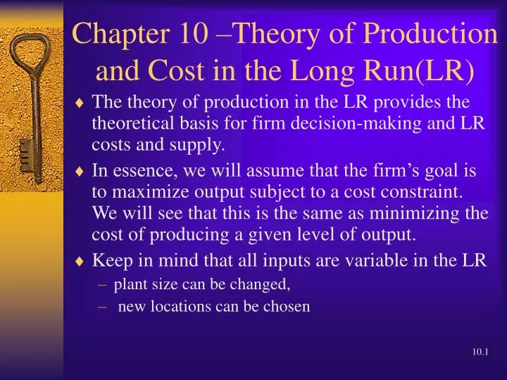
Chapter 10 –Theory of Production and Cost in the Long Run(LR). The theory of production in the LR provides the theoretical basis for firm decision-making and LR costs and supply.

E N D
Chapter 10 –Theory of Production and Cost in the Long Run(LR) • The theory of production in the LR provides the theoretical basis for firm decision-making and LR costs and supply. • In essence, we will assume that the firm’s goal is to maximize output subject to a cost constraint. We will see that this is the same as minimizing the cost of producing a given level of output. • Keep in mind that all inputs are variable in the LR • plant size can be changed, • new locations can be chosen
Production Isoquants • An isoquant is a locus of points indicating different combinations of 2 inputs each of which yields the same level of output. • Note 2 inputs are assumed since we desire to present model graphically.
Characteristics of Isoquants • Negative slope – tradeoffs, if more of L then less of K if output is held constant • Convex to the origin – diminishing MRTS, the more of L you have relative to K the more able you are to trade L for K and hold output constant. • Isoquants cannot intersect
Marginal Rate of Technical Substitution • The MRTS is the (negative of the) slope of the isoquant. Therefore it reflects It is a measure of the number of units of K that must be given up if L is increased by a single unit, holding output constant. Note it will diminish as we move down an isoquant.
Concept of an Isoquant Map • Graph of several isoquants each representing different levels of output. • The higher (further from the origin) an isoquant, the greater the level of output.
Marginal Product and MRTS • Marginal product of an input is the change in total product in response to increasing the variable input by a single unit. • The change in total product is given by the following equation
Marginal Product and MRTS Along an isoquant the change in output is equal to zero and
The Cost Constraint – Isocost Lines • Suppose you have $100, C, to spend on two inputs , L & K, and the prices of each are $10, PL, and $20, PK, respectively. Determine the equation relating K to L reflecting your budget constraint. • 100 = 10L+20K or • K=5-0.5L • In general, the cost constraint is • K = C/PK-(PL/PK)L • Note linear and slope is ratio of prices
Changes in Isocost • What happens to the isocost if cost, C, changes? • What happens to budget line if one of the prices change? • K = C/PK-(PL/PK)L, w=PL, r=PK,C-bar = cost level then isocost is
Change in Cost Budget line I – C=100, PX=10, PY=20 Budget Line II – C=140, Prices same Y 7 5 I 14 10 X
Change in Price Isocost I – C=100, PL=10, PK=20 Isocost II – C=100, PL=20, PK=20 K 7 5 I II 14 10 5 L
Determining the Optimal Combination of Inputs • Producer’s goal is to maximize profits: • Minimize cost of producing a constant level of output • Maximize output subject to a cost constraint • The isocost line shows what combinations of L and K that the producer is able to purchase with a fixed cost level. • The isoquant map shows the producer’s preferences for X and Y.
Minimizing Cost of Producing a Given Level of Output • The Optimal Solution, where the producer minimizes cost subject to an output constraint, is found where the isocost line is tangent to an isoquant. Since isoquants cannot intersect this will be the highest possible level of utility given the constraint. • See Figure 10.4 page 366.
Cost Minimization • At any tangency point the slopes of the two relationships must be equal. • Slope of isoquant is the MRTS – the rate the producer is willing to substitute K for L, holding output constant. • Slope of isocost line is the ratio of prices, PL/PK, which reflects the rate the producer is able to substitute K for L and maintain constant cost.
Cost Minimization Rate willing to sub = Rate able to sub
Cost Minimization • Recall the Marginal Product interpretation of the MRTS or slope of the isoquant. Note PL = w and PK = r in text.
Equilibrium for the Firm • A producer is hiring 20 units of labor and 6 units of capital (bundle A). The price of labor is $10, the price of capital is $2, and at A, the marginal products of labor and capital are both equal to 20. • Is the firm in equilibrium? • No, MP to price ratios are not equal, should use more capital and less labor. • Beginning at A, what happens to output and cost if the producer increases labor by one unit and decreases capital by 1 unit? • Output remains constant and cost increases by $8.
Equilibrium for the Firm • A producer is hiring 20 units of labor and 6 units of capital (bundle A). The price of labor is $10, the price of capital is $2, and at A, the marginal products of labor and capital are both equal to 20. • In equilibrium, which of the following will be true? • MPL will be less than 20. • MPK will be more than 20. • MPL will be 5 times MPK.
Expansion Path • An expansion path is a curve that shows the least costly combination of two inputs required to produce each level of output, holding the input price ratio constant. • See Figure 10.6, page 373. • Along an expansion path,
Expansion Path The following is always true along an expansion path.
Cost Curve Derived from Expansion Path • Since the Expansion Path plots points the optimal combination of inputs required to produce each level of output, total cost for each level of output can be determined since it is assumed that the prices of inputs are fixed. • Thus, if the optimal quantity of labor and capital to produce 100 units of output are 10 and 5 respectively, and the wage rate is $20 and price of capital, $50 then the total cost is $20(10) + $50(5) = $450
Returns to Scale • Returns to Scale deals with the impact on output of a change in the scale(proportional changes in all inputs) of a firm’s operations. • Returns to scale can be classified as • Constant: output changes proportionately to the change in the inputs • Increasing: output changes more than proportionate to the change in the inputs • Decreasing: output changes less than proportionate to the change in the inputs
Returns to Scale • Recall the general form of our production function is Q = f(L,K). Now, suppose we increase all inputs by the factor c as represented in the following production function, F(cL, cK) = zQ • What are the returns to scale if • z = c ? • z > c ? • z < c ?
Long Run Costs • The long run average, LAC, and marginal, LMC, cost curves have the same basic shape that the equivalent short run cost curves. • However, the reason why each is U-shaped is for different reasons, which are • Short run – the Law of Diminishing Marginal returns • Long run – economies/diseconomies of scale
Economies of Scale • Economies of Scale exist when LAC decreases as output increases. • Diseconomies of Scale exist when LAC increases as output increases. LAC diseconomies economies Q
Economies of Scale • Reasons for economies of scale are • Specialization and division of labor • Better meshing of equipment • Economies on capital purchases – machines that are 10 times as productive may not cost 10 times as much • More capital intensive • Reason for diseconomies of scale • Inefficiency in management
Economies of Scope • Scope economies exist if the joint costs of producing two or more products is less than the separate costs of producing each individually. • An example might be an auto air conditioning repair shop that adds radiator/cooling system repairs
Relationship between SR and LR Cost Curves • The LAC curve is a locus of points on SAC curves, which represent the most efficient (cost effective) way of producing each level of output given that the firm has the opportunity and ability to change the quantity of any and all inputs. • See Figure 10.14 page 391.