Download
1 / 37
370 likes | 373 Views
Analysis of Atmospheric Neutrinos: AMANDA 2000-2006. John Kelley April 30, 2008 IceCube Collaboration Meeting. Outline. Hypotheses Analysis Methodology Systematic Errors Data Sample Sensitivities. Figure from Los Alamos Science 25 (1997). Hypotheses.

E N D
Analysis of Atmospheric Neutrinos: AMANDA 2000-2006 John Kelley April 30, 2008 IceCube Collaboration Meeting
Outline • Hypotheses • Analysis Methodology • Systematic Errors • Data Sample • Sensitivities Figure from Los Alamos Science 25 (1997)
Hypotheses • New physics (high-energy flavor-changing phenomena) • violation of Lorentz invariance • quantum decoherence • Conventional theory • measure normalization, spectral slope relative to current models (Bartol, Honda 2006)
New Physics Violation of Lorentz Invariance (VLI) • occurs naturally in many quantum gravity theories • phenomenologically modeled via effective field theory: Standard Model Extension (SME)* • specific form we are interested in: neutrinos have distinct maximum velocity eigenstates ≠ c, and difference c/c results in oscillations * Colladay and Kostelecký, PRD 58 116002 (1998)
VLI + Atmospheric Oscillations • For atmospheric , conventional oscillations turn off above ~50 GeV (L/E dependence) • VLI oscillations turn on at high energy (L E dependence), depending on size of c/c, and distort the zenith angle / energy spectrum (other parameters: mixing angle , phase ) González-García, Halzen, and Maltoni, hep-ph/0502223
VLI Atmospheric Survival Probability maximal mixing, c/c = 10-27
Quantum Decoherence (QD) • Another possible low-energy signature of quantum gravity: quantum decoherence • Heuristic picture: foamy structure of space-time (interactions with virtual black holes) may not preserve certain quantum numbers (like flavor) • Pure states interact with environment and decohere to mixed states
Decoherence + Atmospheric Oscillations characteristic exponential behavior 1:1:1 ratio after decoherence derived from Barenboim, Mavromatos et al. (hep-ph/0603028) Energy dependence depends on phenomenology: n = 3Planck-suppressed operators‡ n = -1 preserves Lorentz invariance n = 2 recoiling D-branes* n = 0 simplest *Ellis et al., hep-th/9704169 ‡ Anchordoqui et al., hep-ph/0506168
Testing the Parameter Space Given observables x, want to determine values of parameters {r} that are allowed / excluded at some confidence level Binned likelihood + Feldman-Cousins excluded c/c allowed sin(2)
Feldman-Cousins Recipe(frequentist construction) • For each point in parameter space {r}, sample many times from parent Monte Carlo distribution (MC “experiments”) • For each MC experiment, calculate likelihood ratio: L =LLH at parent {r} - minimum LLH at some {r,best}(compare hypothesis at this point to best-fit hypothesis) • For each point {r}, find Lcritat which, say, 90% of the MC experiments have a lower L • Once you have the data, compare Ldatato Lcritat each point to determine exclusion region Feldman & Cousins, PRD 57 7 (1998)
Nuisance Parameters / Systematic Errors How to include nuisance parameters {s}: • test statistic becomes profile likelihood • MC experiments use “worst-case” value of nuisance parameters (Feldman’s profile construction method) • specifically, for each r, generate experiments fixing n.p. to data’s , then re-calculate profile likelihood as above
Specifics of the Analysis • Observables (x) • cos(ZenithPandel), [-1, 0], 10 bins • Nch, [20, 120], 10 bins • Physics: parameters of interest (r) • VLI: c/c, sin 2, cos • QD: 3 and 8, 6 and 7 • Nuisance parameters (s) … time for systematics study • must try and limit dimensionality (already 2- or 3-dimensional space to search) • still want to account for shape effects on zenith, Nch — not just normalization
Atmospheric Systematics • Separate systematic errors into four classes, depending on effect on observables: • normalization • e.g. atm. flux normalization • slope: change in primary spectrum • e.g. primary CR slope • tilt: tilts zenith angle distribution • e.g. /K ratio • OM sensitivity (large, complicated effects)
Systematics List error type size method • atm. flux model norm. ±18% MC study • , - scattering angle norm. ±8% MC study • reconstruction bias norm. -4% MC study • -induced muons norm. +2% MC study • charm contribution norm. +1% MC study • timing residuals norm. ±2% 5-year paper • energy loss norm. ±1% 5-year paper rock density norm. <1% MC study primary CR slope (incl. He) slope = ±0.03 Gaisser et al. charm (slope) slope = +0.05 MC study /K ratio tilt tilt +1/-3% MC study charm (tilt) tilt tilt -3% MC study OM sensitivity, ice OM sens. sens. ±10% MC, downgoing
side note: effect of mass-induced neutrino oscillations is O(1%) Atmospheric Flux Models Norm. difference between Bartol, Honda2006: -7% But difference in : -18%; 1/3 -bar: +11%
OM Sensitivity shape normalization slope: 2.5% in norm. / 1% in sens. Unfortunately not possible to parametrize all effects on observables (I tried) new simulation for every year + sensitivity (above right plot is 63 sets)!
Study with atmospheric muons • Compare muon rate in data (trigger level + cleaning) with AHA simulation at various OM sensitivities • Error band on normalization from spread in hadronic models (EPOS, QGSJET-II, and Sibyll) • Pull out a range of allowed OM sensitivities and a mean for this ice model
Estimated Error OM sensitivity (AHA) 85% +10%/-7% EPOS SIBYLL • Zeuthen estimate using atm. zenith angle shape: 100% +3%/-10% (PTD/MAM) • Error spread is close via two methods (17% here vs. 13% Zeuthen) • Difference in mean is from ice model QGSJET-II
Ice Models • Millennium + 100% OM, AHA + 100% OM: both have too much light (at least with v1.54-caustic) • Turn down OM sensitivity to correct muon rate (also fixes neutrino simulation), combine ice + OM errors Atm. vs. PTD/MAM: Millennium +39%AHA +23% AHA (85% OMs) -8%
Ice Model Uncertainty Covered by 10% in OM sensitivity (roughly same uncertainty as muon analysis)
Pion/Kaon Ratio Change /K ratio using Gaisser formulation: uncertainty in ZN, ZNK*: AK/A [0.28,0.51] shape difference tilt function tilt +1%/-3% cos(zenith) *Agrawal et al., PRD 53 (1996)
Spectral Slope • Uncertainty in primary CR slope dominated by He: He = 0.07*to first order: p + fHe He = 0.03 • Tweak atmospheric model by (E/Emedian), Emedian = 630 GeV • Other uncertainties (charm) increase range of *Gaisser, Honda et al., 2001 ICRC
7-year Data Sample • 2000-2006 data • 2000-04: Zeuthen combined filtering • 2005-06: Madison filtering • 1387 days livetime • Zeuthen final cuts • purity is important (small unsimulated b.g.) • not specifically optimized for high energy • after cuts: 6099 events below horizon (4.4/day) • rate similar to 4-year Mainz sample (4.2/day) • Nch, zenith angle removed from files until unblinding
VLI Sensitivity • 2000-03 analysis (Ahrens): c/c < 5.3 10-27 (90%CL) • Median sensitivity (2 approx.): c/c < 4.3 10-27 (90%CL) • Sample sensitivity (1 MC experiment, full construction): c/c < 4.5 10-27 (90%CL) excluded excluded best fit 90%, 95%, 99% allowed CL (maximal mixing, cos = 0)
QD Sensitivity • ANTARES sensitivity (3 years)*:* < 2 10-30 GeV-1 (2-flavor) • This analysis (1 MC experiment, full construction): * < 2.0 10-31 GeV-1 excluded best fit 90%, 95%, 99% allowed CL (E2 model, 3 = 8 = 6 = 7) * Morgan et al., astro-ph/0412618
Conventional Analysis • Parameters of interest: normalization, slope change • Nuisance parameters: remove atm. flux norm. and slope uncertainty, keep others • Sensitivity: roughly ±15% in normalization, ±0.07 in slope MC test: Bartol input best fit best fit 90%, 95%, 99% allowed
Energy Spectrum • Allowed band: range of parameters from previous plot • Energy range: intersection of 5-95% regions, MC final cut level, various OM sens. • With data: will use both Bartol and Honda as reference shapes, allowed regions should be similar
On the Docket • May add E3 decoherence, E2 VLI • analysis procedure the same, just computation time • Possible mid-to-high-Nch excess in data • discussion violates blindness, but excess would be inconsistent with any proposed new physics hypothesis • will design two-step unblinding procedure to address any serious contamination • Unblinding request out to working group very shortly!
Analysis Methodology: Binned Likelihood Test Poisson probability Product over bins example of sampling / LLH comparison Test Statistic: LLH
Optimal Binning • In general: finer binning is always better for LLH analysis • But gain after a certain point is nominal, could run into data/MC artifacts • Use 10 bins in each observable
Computational Details • Weighted MC observable histograms precomputed on a grid in {r, s} space (r more finely binned) • ~2min./histogram x 16k-32k points/hypothesis = 1 CPU-month / hypothesis • 1000 MC experiments per point in {r} space • likelihood minimization over {r, s} exhaustive search because of discrete parameter space • construction: about 12h / hypothesis (still manageable) • Recording confidence level at each point (instead of just yes/no at a CL) allows some contour interpolation
MC Sample(s) • nusim: zenith range (80,180) with =1.5 • Amasim Aluminum-opt5 + AHA ice (v1) + Photonics 1.54-caustic • (9 periods) x (7 OM sens.) = 63 MC sets • everything else via weighting • For atm. neutrinos: ~60 years of effective livetime at each OM sensitivity